Top 1 Kaggle – My best method and how to use

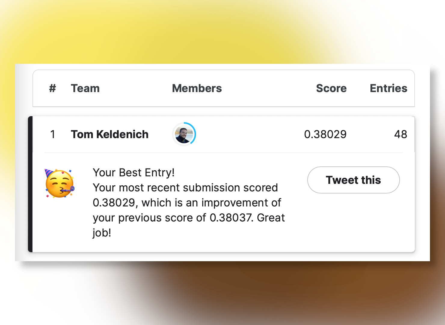
On April 04, 2023, I reached TOP 1 in a Kaggle competition ranking. I share everything with you in this article!

Kaggle is a website that allows anyone to participate in Machine Learning competitions.

The goal is simple: build the best Machine Learning model to solve a given problem.

Kaggle brings together beginners in Artificial Intelligence and the most advanced people in the field.

This is how we can see experts from big AI companies like Nvidia, Google, Facebook… and simple university students challenging each other!

In this article, I’ll guide you through the code that allowed me to reach the first position in the Store Sales – Time Series Forecasting.

By exploring this code, you will be able to copy it and reach the top of the ranking… or even improve it to beat me!

So why am I sharing this code with you if I’m going to lose my ranking?

First of all, because I like open source and the idea that everyone can access the information.

Second, because this competition is in the Getting Started category anyway. This implies that the ranking is renewed every 3 months. But above all, that there is no deadline to participate in this challenge.

The progress in AI being what it is, it is obvious that my record will be beaten in the months or years to come. So, instead of constraining this progress, why not encourage it by sharing my code?

Anyway, that being said, for the sake of history (and honestly for my ego) I have recorded the ranking of April 04, 2023:

How I did it

To reach the first place I inspired myself from Ferdinand Berr’s code, adding some changes to it.

First I modified the hyperparameters of the model he uses. Then I added a basic improvement technique that seems to have been neglected in this competition: the Ensemble Method.

The idea is to combine the predictions of several models and to average them to obtain an optimal result. I detail the method in this article.

The objective of this competition is to predict the number of sales that different stores located in Ecuador will generate.

To make these predictions, we’ll have to rely on the past sales of the stores.

This type of variable is called a time series.

A time series is a sequence of data measured at regular intervals in time.

In our case, the data was recorded every day.

In the following I will detail the code I used. I have removed the extra information that was not helpful to the understanding to keep only the essential. You’ll see that the code is more airy than in the solution I used as a basis.

This tutorial is aimed at people with an intermediate level in AI, even if it can also be approached by beginners.

We will combine several data and use a little known but powerful Machine Learning library for our task: darts.

Darts allows to manipulate and predict the values of a time series easily.

Without further introduction, let’s get to work!

Data

First of all I propose to explore the dataset.

Our goal is to predict future sales of stores located in Ecuador, for the dates August 16, 2017 to August 31, 2017 (16 days).

In our dataset, there are 54 stores for 33 product families.

We need to predict the sales for each of these product families from each store. So 33 * 54 * 16 = 28,512 values to predict.

If you work on a notebook, you can load the dataset with this line of code:

!git clone https://github.com/tkeldenich/datasets.git
!unzip /content/datasets/store-sales-time-series-forecasting.zip -d /content/datasets/

To help us make the predictions, no less than 8 CSV files are provided.

Let’s display them to better understand our job.

train.csv

First of all the main file: train.csv. It contains some features and the label to predict sales, the number of sales per day:

import pandas as pd

df_train = pd.read_csv('/content/datasets/store-sales-time-series-forecasting/train.csv')
display(df_train.head())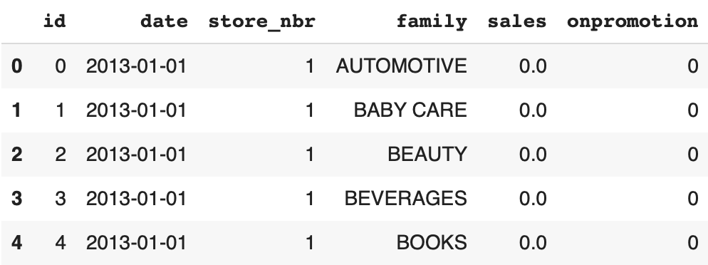

Here are the columns of the DataFrame:

• id – the index of the row
• date – the current date
• store_nbr – the store
• family – the product family
• sales – number of sales in this family
• onpromotion – the number of products on promotion in this family

holidays_events.csv

The holidays_events.csv groups the national holidays. This information is independent of the store but can have an impact on sales.

For example, on a holiday, there might be more people in the city and therefore more customers in the stores. Or conversely, more people might go on vacation and therefore there would be fewer customers in the stores.

df_holidays_events = pd.read_csv('/content/datasets/store-sales-time-series-forecasting/holidays_events.csv')
display(df_holidays_events.head())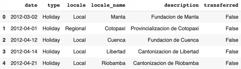

Here are the columns in the DataFrame:

• date – the date of the holiday
• type – the type of holiday (Holiday, Event, Transfer (see transferred column), Additional, Bridge, Work Day)
• locale – the scope of the event (Local, Regional, National)
• locale_name – the city where the event takes place
• description – name of the event
• transferred – whether the event has been transferred (moved to another day) or not

oil.csv

Then a CSV file gathers the daily oil price from January 01, 2013 to August 31, 2017:

df_oil = pd.read_csv('/content/datasets/store-sales-time-series-forecasting/oil.csv')
display(df_oil.head())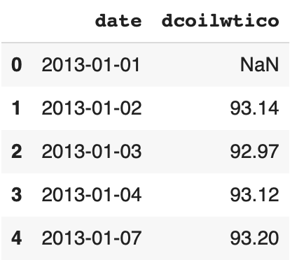

store.csv

The store.csv file gathers information about the stores. There is one store per line so 54 lines:

df_stores = pd.read_csv('/content/datasets/store-sales-time-series-forecasting/stores.csv')
display(df_stores.head())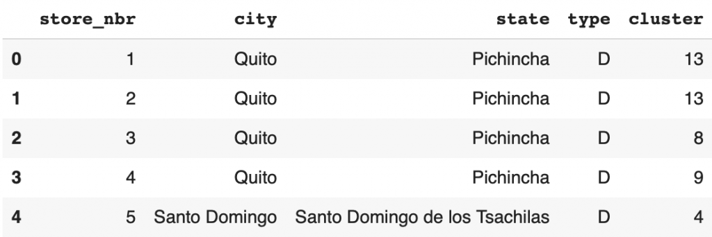

DataFrame columns:

• store_nbr – the store
• city – the city where the store is located
• state – the state where the store is located
• type – the type of the store
• cluster – the number of similar stores in the vicinity

transactions.csv

The transactions.csv file groups the daily transactions by stores:

df_transactions = pd.read_csv('/content/datasets/store-sales-time-series-forecasting/transactions.csv')
display(df_transactions.head())

Note: a transaction is a receipt created after a customer’s purchase

test.csv

Finally, we have the test.csv that will allow us to predict the sales column. The file starts on August 16, 2017 and ends on August 31, 2017. We also have the sample_submission.csv to fill in with the number of sales per day and per family:

df_test = pd.read_csv('/content/datasets/store-sales-time-series-forecasting/test.csv')
df_sample_submission = pd.read_csv('/content/datasets/store-sales-time-series-forecasting/sample_submission.csv')
display(df_test.head())
display(df_sample_submission.head())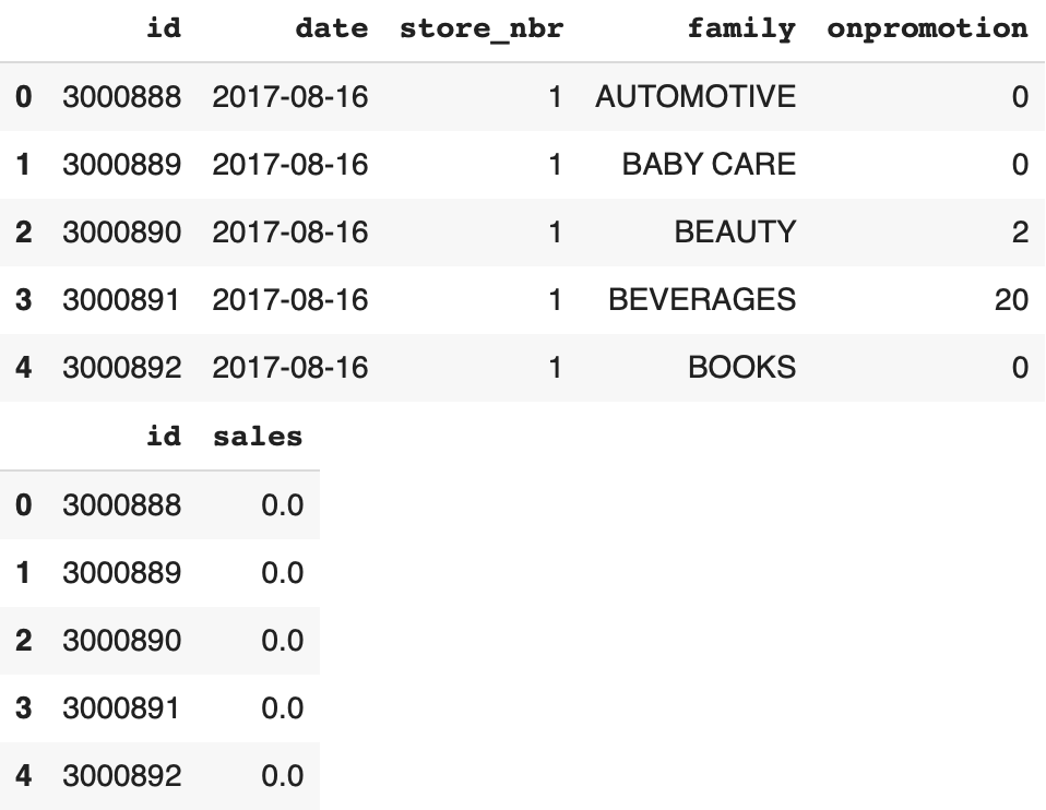

The test.csv contains 5 columns:

• id – the index of the row (which will be used to fill in the sample_submission.csv file)
• date – the current date
• store_nbr – the store
• family – the product family
• sales – the number of sales in this family
• onpromotion – the number of products on promotion in this family

Now that we know our dataset better, we can move on to the preprocessing step which will allow us to format our data to train our Machine Learning model.

Preprocessing

To start the preprocessing, let’s group the name of each product family and the number of each store:

family_list = df_train['family'].unique()
store_list = df_stores['store_nbr'].unique()
display(family_list)
display(store_list)

Output :

array(['AUTOMOTIVE', 'BABY CARE', 'BEAUTY', 'BEVERAGES', 'BOOKS', 'BREAD/BAKERY', 'CELEBRATION', 'CLEANING', 'DAIRY', 'DELI', 'EGGS', 'FROZEN FOODS', 'GROCERY I', 'GROCERY II', 'HARDWARE', 'HOME AND KITCHEN I', 'HOME AND KITCHEN II', 'HOME APPLIANCES', 'HOME CARE', 'LADIESWEAR', 'LAWN AND GARDEN', 'LINGERIE', 'LIQUOR,WINE,BEER', 'MAGAZINES', 'MEATS', 'PERSONAL CARE', 'PET SUPPLIES', 'PLAYERS AND ELECTRONICS', 'POULTRY', 'PREPARED FOODS', 'PRODUCE', 'SCHOOL AND OFFICE SUPPLIES', 'SEAFOOD'], dtype=object)

array([ 1,  2,  3,  4,  5,  6,  7,  8,  9, 10, 11, 12, 13, 14, 15, 16, 17, 18, 19, 20, 21, 22, 23, 24, 25, 26, 27, 28, 29, 30, 31, 32, 33, 34, 35, 36, 37, 38, 39, 40, 41, 42, 43, 44, 45, 46, 47, 48, 49, 50, 51, 52, 53, 54])

Next, we assemble the df_train and df_stores datasets. By grouping this dat in a single dataset, it will allow us to access the information more easily. In addition to that, we sort the sales of the DataFrame by date, by family and by stores:

train_merged = pd.merge(df_train, df_stores, on ='store_nbr')
train_merged = train_merged.sort_values(["store_nbr","family","date"])
train_merged = train_merged.astype({"store_nbr":'str', "family":'str', "city":'str',
                          "state":'str', "type":'str', "cluster":'str'})

display(train_merged.head())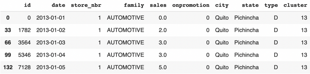

A time series being the number of sales made per day for a family of a store, this sorting will allow us to extract them more easily.

Same thing for the test DataFrame, we sort the sales by date, by family and by stores:

df_test_dropped = df_test.drop(['onpromotion'], axis=1)
df_test_sorted = df_test_dropped.sort_values(by=['store_nbr','family'])

display(df_test_sorted.head())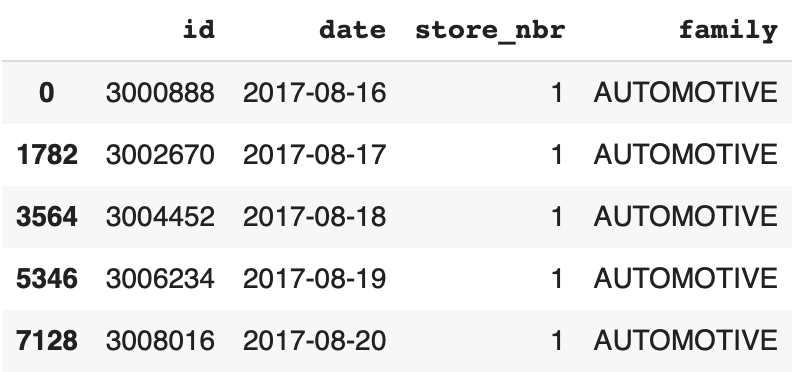

Now we are going to concretely create time series!

Main Time Series

As I mentioned earlier, we are going to use a specific library for time series processing in Python: Darts.

Darts allows us to easily manipulate time series.

I invite you to install the darts library:

!pip install darts==0.23.1

Like Pandas with its DataFrame, the Darts library offers us its class allowing to manipulate time series : the TimeSeries.

We will use these class to extract our time series.

But before that, we have to discuss our strategy.

Strategy

Reminder: Our objective is to predict for each family in each store the number of future sales. There are 33 families for 54 stores.

From there, several routes can be taken.

The most obvious one is to train a Machine Learning model on our dataset. On the 1782 time series.

This is obvious because it allows us to use a maximum of data to train our model. It will then be able to generalize its knowledge to each of the product families. With such a strategy, our model will have a good global prediction.

A less obvious strategy, but quite logical, is to train a Machine Learning model for each time series.

Indeed, by assigning a model to each series, we ensure that each model is specialized in its task and therefore performs well in its prediction, and this for each product family of each store.

The problem with the first method is that the model, having only a general knowledge of our data, will not have an optimal prediction on each specific time series.

The problem with the second method is that the model will be specialized on each time series, but will lack data to perfect its training.

We will therefore not take any of the strategies described above.

Our strategy is to position ourselves between these two methods.

After several tests and analyses of our data (which I will not detail here), we understand that the sales by families seem to be correlated across stores.

Hence we’ll train a Machine Learning model by product family.

We will have 33 models, each trained on 54 time series.

This is a good compromise, because it allows us to have a lot of data to train a model. But also to obtain, at the end of the training, a model specialized in its task (because trained on a single product family).

Now that you know the strategy, let’s implement it!

sales

Extract the time series

For each product family, we will gather all the time series concerning it.

So we will have 33 sub-datasets. These datasets will be contained in the family_TS_dict dictionary.

In the following lines of code, we extract the TimeSeries of the 54 stores for each family.

These TimeSeries will group the sales by family, the date of each sale, but also the dependent covariates (indicated with group_cols and static_cols) of these sales: store_nbr, family, city, state, type, cluster :

import numpy as np
import darts
from darts import TimeSeries

family_TS_dict = {}

for family in family_list:
  df_family = train_merged.loc[train_merged['family'] == family]

  list_of_TS_family = TimeSeries.from_group_dataframe(
                                df_family,
                                time_col="date",
                                group_cols=["store_nbr","family"],
                                static_cols=["city","state","type","cluster"],
                                value_cols="sales",
                                fill_missing_dates=True,
                                freq='D')
  for ts in list_of_TS_family:
            ts = ts.astype(np.float32)

  list_of_TS_family = sorted(list_of_TS_family, key=lambda ts: int(ts.static_covariates_values()[0,0]))
  family_TS_dict[family] = list_of_TS_family

You can also see that we indicate fill_missing_dates=True because in the dataset, the sales of each December 25th are missing.

We also indicate freq='D', to indicate that the interval for the values of the time series is in days (D for day).

Finally, we indicate that the values of the TimeSeries must be interpreted in float32 and that the time series must be sorted by stores.

We can display the first time series of the first family:

display(family_TS_dict['AUTOMOTIVE'][0])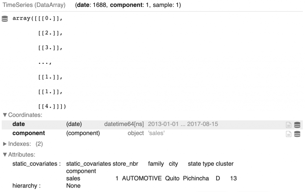

We retrieve all the values indicated above: the number of sales, the date of each sale in Coordinates > date, and the dependent covariates in Attributes > static_covariates.

You can also see that the length of the time series is 1688. Originally it was 1684 but we added the values of the four December 25s that are missing from the dataset.

Then we apply a normalization to our TimeSeries.

Normalizing time series

Normalization is a technique used to improve the performance of a Machine Learning model by facilitating its training. I let you refer to our article on the subject if you want to know more.

We can easily normalize a TimeSeries with the Scaler function of darts.

Moreover, we will further optimize the training of the model by one hot encoding our covariates. We implement the one hot encoding via the StaticCovariatesTransformer function.

from darts.dataprocessing import Pipeline
from darts.dataprocessing.transformers import Scaler, StaticCovariatesTransformer, MissingValuesFiller, InvertibleMapper
import sklearn

family_pipeline_dict = {}
family_TS_transformed_dict = {}

for key in family_TS_dict:
  train_filler = MissingValuesFiller(verbose=False, n_jobs=-1, name="Fill NAs")
  static_cov_transformer = StaticCovariatesTransformer(verbose=False, transformer_cat = sklearn.preprocessing.OneHotEncoder(), name="Encoder")
  log_transformer = InvertibleMapper(np.log1p, np.expm1, verbose=False, n_jobs=-1, name="Log-Transform")   
  train_scaler = Scaler(verbose=False, n_jobs=-1, name="Scaling")

  train_pipeline = Pipeline([train_filler,
                             static_cov_transformer,
                             log_transformer,
                             train_scaler])
     
  training_transformed = train_pipeline.fit_transform(family_TS_dict[key])
  family_pipeline_dict[key] = train_pipeline
  family_TS_transformed_dict[key] = training_transformed

We can display the first transformed TimeSeries of the first family:

display(family_TS_transformed_dict['AUTOMOTIVE'][0])

You can see that the sales have been normalized and that the static_covariates have been one hot encoded.

We now have our main time series that will allow us to train our model.

Why not expand our dataset with other covariates?

Covariates

A covariate is a variable that helps to predict a target variable.

This covariate can be dependent on the target variable. For example, the type of store, type, where the sales are made. But it can also be independent. For example, the price of oil on the day of the sale of a product.

This covariate can be known in advance, for example in our dataset we have the price of oil from January 1, 2013 to August 31, 2017. In this case, we talk about a future covariate.

There are also past covariates. These are covariates that are not known in advance. For example in our dataset, the transactions are known for the dates January 1, 2013 to August 15, 2017.

Date

The first covariate we are interested in is the date.

The date is a future covariate because we know the date of the coming days.

It has, in many cases, an impact on the traffic of a store. For example, we can expect that on Saturday there will be more customers in the store than on Monday.

But it can also be expected that during the summer vacations the store will be less busy than in normal times.

Hence every little detail counts.

In order not to miss anything, we will extract as much information as possible from this date. Here, 7 columns :

• year – year
• month – month
• day – day
• dayofyear – day of the year (for example February 1 is the 32nd day of the year)
• weekday – day of the week (there are 7 days in a week)
• weekofyear – week of the year (there are 52 weeks in a year)
• linear_increase – the index of the interval

from darts.utils.timeseries_generation import datetime_attribute_timeseries

full_time_period = pd.date_range(start='2013-01-01', end='2017-08-31', freq='D')


year = datetime_attribute_timeseries(time_index = full_time_period, attribute="year")
month = datetime_attribute_timeseries(time_index = full_time_period, attribute="month")
day = datetime_attribute_timeseries(time_index = full_time_period, attribute="day")
dayofyear = datetime_attribute_timeseries(time_index = full_time_period, attribute="dayofyear")
weekday = datetime_attribute_timeseries(time_index = full_time_period, attribute="dayofweek")
weekofyear = datetime_attribute_timeseries(time_index = full_time_period, attribute="weekofyear")
timesteps = TimeSeries.from_times_and_values(times=full_time_period,
                                             values=np.arange(len(full_time_period)),
                                             columns=["linear_increase"])

time_cov = year.stack(month).stack(day).stack(dayofyear).stack(weekday).stack(weekofyear).stack(timesteps)
time_cov = time_cov.astype(np.float32)

This is what it gives us for the date at index 100:

display(print(time_cov.components.values))
display(time_cov[100])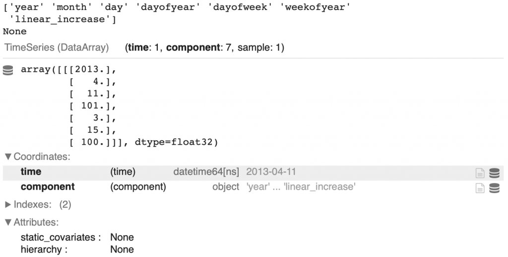

And of course, we will normalize this data:

time_cov_scaler = Scaler(verbose=False, n_jobs=-1, name="Scaler")
time_cov_train, time_cov_val = time_cov.split_before(pd.Timestamp('20170816'))
time_cov_scaler.fit(time_cov_train)
time_cov_transformed = time_cov_scaler.transform(time_cov)

You can also see that a split is made between the dates before August 15, 2017 and after (dates that will be used in the prediction).

Oil

As said before, the price of oil is a future covariate because it is known in advance.

Here, we will not simply extract the daily oil price but we will calculate the moving average.

The moving average in X, is an average of the current value and the X-1 previous values of a time series.

For example the moving average in 7 is the average of (t + t-1 + … + t-6) / 7. It is calculated at each t, that’s why it is called “moving”.

Calculating the moving average allows us to remove the momentary fluctuations of a value and thus to accentuate the long-term trends.

The moving average is used in trading, but more generally in Time Series Analysis.

In the following code, we calculate the moving average in 7 and 28 of the oil price. And of course, we apply a normalization :

from darts.models import MovingAverage
# Oil Price

oil = TimeSeries.from_dataframe(df_oil, 
                                time_col = 'date', 
                                value_cols = ['dcoilwtico'],
                                freq = 'D')

oil = oil.astype(np.float32)

# Transform
oil_filler = MissingValuesFiller(verbose=False, n_jobs=-1, name="Filler")
oil_scaler = Scaler(verbose=False, n_jobs=-1, name="Scaler")
oil_pipeline = Pipeline([oil_filler, oil_scaler])
oil_transformed = oil_pipeline.fit_transform(oil)

# Moving Averages for Oil Price
oil_moving_average_7 = MovingAverage(window=7)
oil_moving_average_28 = MovingAverage(window=28)

oil_moving_averages = []

ma_7 = oil_moving_average_7.filter(oil_transformed).astype(np.float32)
ma_7 = ma_7.with_columns_renamed(col_names=ma_7.components, col_names_new="oil_ma_7")
ma_28 = oil_moving_average_28.filter(oil_transformed).astype(np.float32)
ma_28 = ma_28.with_columns_renamed(col_names=ma_28.components, col_names_new="oil_ma_28")
oil_moving_averages = ma_7.stack(ma_28)

Here is the result obtained at index 100:

display(oil_moving_averages[100])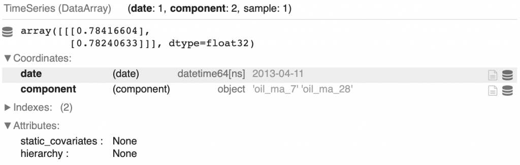

Holidays

Let’s now focus on the holidays.

Here, Ferdinand Berr has implemented functions to detail these holidays. In particular, he adds information about whether the holiday is Christmas day, whether it is a soccer game day, etc:

def holiday_list(df_stores):

    listofseries = []
    
    for i in range(0,len(df_stores)):
            
            df_holiday_dummies = pd.DataFrame(columns=['date'])
            df_holiday_dummies["date"] = df_holidays_events["date"]
            
            df_holiday_dummies["national_holiday"] = np.where(((df_holidays_events["type"] == "Holiday") & (df_holidays_events["locale"] == "National")), 1, 0)

            df_holiday_dummies["earthquake_relief"] = np.where(df_holidays_events['description'].str.contains('Terremoto Manabi'), 1, 0)

            df_holiday_dummies["christmas"] = np.where(df_holidays_events['description'].str.contains('Navidad'), 1, 0)

            df_holiday_dummies["football_event"] = np.where(df_holidays_events['description'].str.contains('futbol'), 1, 0)

            df_holiday_dummies["national_event"] = np.where(((df_holidays_events["type"] == "Event") & (df_holidays_events["locale"] == "National") & (~df_holidays_events['description'].str.contains('Terremoto Manabi')) & (~df_holidays_events['description'].str.contains('futbol'))), 1, 0)

            df_holiday_dummies["work_day"] = np.where((df_holidays_events["type"] == "Work Day"), 1, 0)

            df_holiday_dummies["local_holiday"] = np.where(((df_holidays_events["type"] == "Holiday") & ((df_holidays_events["locale_name"] == df_stores['state'][i]) | (df_holidays_events["locale_name"] == df_stores['city'][i]))), 1, 0)
                     
            listofseries.append(df_holiday_dummies)

    return listofseries

Then, we have a function to remove the days equal to 0 and the duplicates:

def remove_0_and_duplicates(holiday_list):

    listofseries = []
    
    for i in range(0,len(holiday_list)):
            
            df_holiday_per_store = list_of_holidays_per_store[i].set_index('date')

            df_holiday_per_store = df_holiday_per_store.loc[~(df_holiday_per_store==0).all(axis=1)]
            
            df_holiday_per_store = df_holiday_per_store.groupby('date').agg({'national_holiday':'max', 'earthquake_relief':'max', 
                                   'christmas':'max', 'football_event':'max', 
                                   'national_event':'max', 'work_day':'max', 
                                   'local_holiday':'max'}).reset_index()

            listofseries.append(df_holiday_per_store)

    return listofseries

And finally a function that allows us to have the holidays associated to each of the 54 stores :

def holiday_TS_list_54(holiday_list):

    listofseries = []
    
    for i in range(0,54):
            
            holidays_TS = TimeSeries.from_dataframe(list_of_holidays_per_store[i], 
                                        time_col = 'date',
                                        fill_missing_dates=True,
                                        fillna_value=0,
                                        freq='D')
            
            holidays_TS = holidays_TS.slice(pd.Timestamp('20130101'),pd.Timestamp('20170831'))
            holidays_TS = holidays_TS.astype(np.float32)
            listofseries.append(holidays_TS)

    return listofseries

Now we just need to apply these functions:

list_of_holidays_per_store = holiday_list(df_stores)
list_of_holidays_per_store = remove_0_and_duplicates(list_of_holidays_per_store)   
list_of_holidays_store = holiday_TS_list_54(list_of_holidays_per_store)

holidays_filler = MissingValuesFiller(verbose=False, n_jobs=-1, name="Filler")
holidays_scaler = Scaler(verbose=False, n_jobs=-1, name="Scaler")

holidays_pipeline = Pipeline([holidays_filler, holidays_scaler])
holidays_transformed = holidays_pipeline.fit_transform(list_of_holidays_store)

We get 54 TimeSeries with 7 columns:

• national_holiday
• earthquake_relief
• christmas
• football_event
• national_event
• work_day
• local_holiday

Here is the TimeSeries index 100 for the first store:

display(len(holidays_transformed))
display(holidays_transformed[0].components.values)
display(holidays_transformed[0][100])

Promotion

The last future covariate to process is the onpromotion column.

It gives us the number of items on promotion in a product family.

Here the code is similar to the one used for the sales column. It allows to extract for each family, the time series of the 54 stores:

df_promotion = pd.concat([df_train, df_test], axis=0)
df_promotion = df_promotion.sort_values(["store_nbr","family","date"])
df_promotion.tail()

family_promotion_dict = {}

for family in family_list:
  df_family = df_promotion.loc[df_promotion['family'] == family]

  list_of_TS_promo = TimeSeries.from_group_dataframe(
                                df_family,
                                time_col="date",
                                group_cols=["store_nbr","family"],
                                value_cols="onpromotion",
                                fill_missing_dates=True,
                                freq='D')
  
  for ts in list_of_TS_promo:
    ts = ts.astype(np.float32)

  family_promotion_dict[family] = list_of_TS_promo

We can display the first TimeSeries of the first family :

display(family_promotion_dict['AUTOMOTIVE'][0])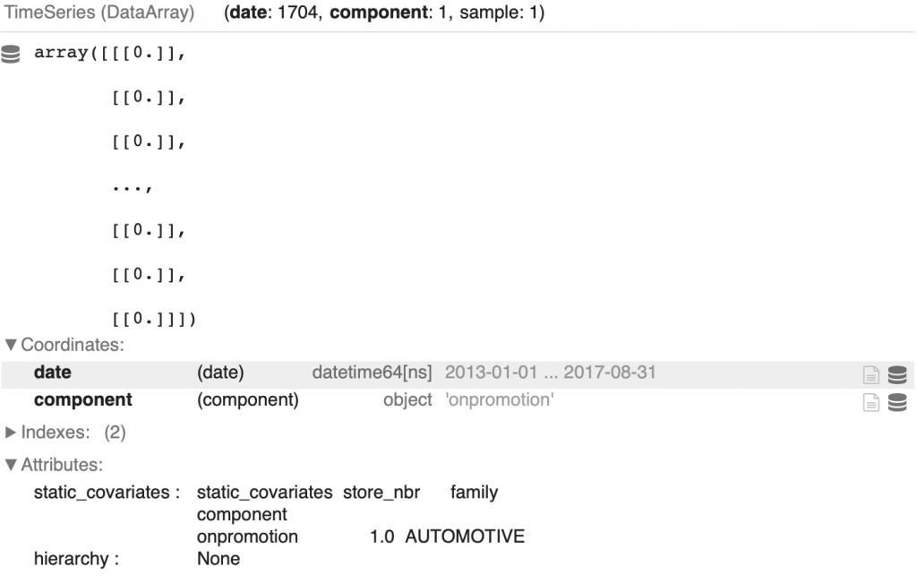

Let’s go further by calculating also the moving average in 7 and 28, like for the oil price:

from tqdm import tqdm

promotion_transformed_dict = {}

for key in tqdm(family_promotion_dict):
  promo_filler = MissingValuesFiller(verbose=False, n_jobs=-1, name="Fill NAs")
  promo_scaler = Scaler(verbose=False, n_jobs=-1, name="Scaling")

  promo_pipeline = Pipeline([promo_filler,
                             promo_scaler])
  
  promotion_transformed = promo_pipeline.fit_transform(family_promotion_dict[key])
  
  # Moving Averages for Promotion Family Dictionaries
  promo_moving_average_7 = MovingAverage(window=7)
  promo_moving_average_28 = MovingAverage(window=28)

  promotion_covs = []

  for ts in promotion_transformed:
    ma_7 = promo_moving_average_7.filter(ts)
    ma_7 = TimeSeries.from_series(ma_7.pd_series())  
    ma_7 = ma_7.astype(np.float32)
    ma_7 = ma_7.with_columns_renamed(col_names=ma_7.components, col_names_new="promotion_ma_7")
    ma_28 = promo_moving_average_28.filter(ts)
    ma_28 = TimeSeries.from_series(ma_28.pd_series())  
    ma_28 = ma_28.astype(np.float32)
    ma_28 = ma_28.with_columns_renamed(col_names=ma_28.components, col_names_new="promotion_ma_28")
    promo_and_mas = ts.stack(ma_7).stack(ma_28)
    promotion_covs.append(promo_and_mas)

  promotion_transformed_dict[key] = promotion_covs

We obtain a normalized time series with 3 columns.

We can display the index 1 of the first TimeSeries of the first family:

display(promotion_transformed_dict['AUTOMOTIVE'][0].components.values)
display(promotion_transformed_dict['AUTOMOTIVE'][0][1])

Grouping the covariates

To finish with the future covariates, we are going to gather them in the same TimeSeries.

We start with the time series of the dates, the oil price and the moving averages of the oil price that we group in the variable general_covariates :

general_covariates = time_cov_transformed.stack(oil_transformed).stack(oil_moving_averages)

Then for each store, we gather the TimeSeries of the holidays with the general_covariates :

store_covariates_future = []

for store in range(0,len(store_list)):
  stacked_covariates = holidays_transformed[store].stack(general_covariates)  
  store_covariates_future.append(stacked_covariates)

Finally, for each family, we combine the previously created covariates with the promotion covariates:

future_covariates_dict = {}

for key in tqdm(promotion_transformed_dict):

  promotion_family = promotion_transformed_dict[key]
  covariates_future = [promotion_family[i].stack(store_covariates_future[i]) for i in range(0,len(promotion_family))]

  future_covariates_dict[key] = covariates_future

Here are the different columns obtained for each TimeSeries of each family of each store:

display(future_covariates_dict['AUTOMOTIVE'][0].components)

Output : ['onpromotion', 'promotion_ma_7', 'promotion_ma_28', 'national_holiday', 'earthquake_relief', 'christmas', 'football_event', 'national_event', 'work_day', 'local_holiday', 'year', 'month', 'day', 'dayofyear', 'dayofweek', 'weekofyear', 'linear_increase', 'dcoilwtico', 'oil_ma_7', 'oil_ma_28']

Transactions – Past Covariates

Before launching the training of the model, let’s extract the past covariates: the transactions.

As you might already have understand, after having taken the transactions for each store, we will normalize them:

df_transactions.sort_values(["store_nbr","date"], inplace=True)

TS_transactions_list = TimeSeries.from_group_dataframe(
                                df_transactions,
                                time_col="date",
                                group_cols=["store_nbr"],
                                value_cols="transactions",
                                fill_missing_dates=True,
                                freq='D')

transactions_list = []

for ts in TS_transactions_list:
            series = TimeSeries.from_series(ts.pd_series())
            series = series.astype(np.float32)
            transactions_list.append(series)

transactions_list[24] = transactions_list[24].slice(start_ts=pd.Timestamp('20130102'), end_ts=pd.Timestamp('20170815'))

from datetime import datetime, timedelta

transactions_list_full = []

for ts in transactions_list:
  if ts.start_time() > pd.Timestamp('20130101'):
    end_time = (ts.start_time() - timedelta(days=1))
    delta = end_time - pd.Timestamp('20130101')
    zero_series = TimeSeries.from_times_and_values(
                              times=pd.date_range(start=pd.Timestamp('20130101'), 
                              end=end_time, freq="D"),
                              values=np.zeros(delta.days+1))
    ts = zero_series.append(ts)
    ts = ts.with_columns_renamed(col_names=ts.components, col_names_new="transactions")
    transactions_list_full.append(ts)

transactions_filler = MissingValuesFiller(verbose=False, n_jobs=-1, name="Filler")
transactions_scaler = Scaler(verbose=False, n_jobs=-1, name="Scaler")

transactions_pipeline = Pipeline([transactions_filler, transactions_scaler])
transactions_transformed = transactions_pipeline.fit_transform(transactions_list_full)

Here is the TimeSeries for the first store:

display(transactions_transformed[0])

We are finally ready to create our Machine Learning model.

Machine Learning Model

Now, we will train a first Machine Learning model with the darts library to confirm that our data is consistent and that the predictions obtained are convincing.

Then we will use ensemble methods to improve our final result.

Single model

The Darts library offers us various Machine Learning models to use on TimeSeries.

In Ferdinand Berr’s solution, we can see that he uses different models:

• NHiTSModel – score : 0.43265
• RNNModel (with LSTM layers) – score : 0.55443
• TFTModel – score : 0.43226
• ExponentialSmoothing – score : 0.37411

These scores are obtained on validation data, artificially generated from the training data.

Personally, I decided to use the LightGBMModel, an implementation of the eponymous library model on which you will find an article here.

Why use this model ? Not after hours of practice and experimentation, but simply by using it and seeing that, alone, it gives me better results than the ExponentialSmoothing.

As explained in the Strategy section, we will train a Machine Learning model for each product family.

So for each family, we have to take the corresponding TimeSeries and send them to our Machine Learning model.

First, we prepare the data:

• TCN_covariates represents the future covariates associated with the target product family
• train_sliced represents the number of sales associated with the target product family. The slice_intersect function that you can see used simply ensures that the components span the same time interval. In the case of different time intervals an error message will appear if we try to combine them.
• transactions_transformed, the past covariates do not need to be indexed on the target family because there is only one global TimeSeries per store

Next, we initialize hyperparameters for our model.

This is the key to model results.

By modifying these hyperparameters you can improve the performance of the Machine Learning model.

Training

Here are the important hyperparameters:

• lags – the number of past values on which we base our predictions
• lags_future_covariates – the number of future covariate values on which we base our predictions. If we give a tuple, the left value represents the number of covariates in the past and the right value represents the number of covariates in the future
• lags_past_covariates – the number of past covariate values on which we base our predictions

For these three hyperparameters, if a list is passed, we take the indexes associated with the numbers of this list. For example if we pass: [-3, -4, -5], we take the indexes t-3, t-4, t-5. But if we pass an integer for example 10, we take the 10 previous values (or the 10 future values depending on the case).

The hyperparameters output_chunk_length controls the number of predicted values in the future, random_state ensures the reproducibility of the results and gpu_use_dp indicates if we want to use a GPU.

After that we launch the training. And at the end, we save the trained model in a dictionary.

from darts.models import LightGBMModel

LGBM_Models_Submission = {}

display("Training...")

for family in tqdm(family_list):

  sales_family = family_TS_transformed_dict[family]
  training_data = [ts for ts in sales_family] 
  TCN_covariates = future_covariates_dict[family]
  train_sliced = [training_data[i].slice_intersect(TCN_covariates[i]) for i in range(0,len(training_data))]

  LGBM_Model_Submission = LightGBMModel(lags = 63,
                                        lags_future_covariates = (14,1),
                                        lags_past_covariates = [-16,-17,-18,-19,-20,-21,-22],
                                        output_chunk_length=1,
                                        random_state=2022,
                                        gpu_use_dp= "false",
                                        )
     
  LGBM_Model_Submission.fit(series=train_sliced, 
                        future_covariates=TCN_covariates,
                        past_covariates=transactions_transformed)

  LGBM_Models_Submission[family] = LGBM_Model_Submission

In the above code, we only use lags_past_covariates = [-16,-17,-18,-19,-20,-21,-22], why? Because during the 16th prediction (the one of August 31, 2017), the values of the past covariates from -1 to -15 are not known.

After training, we obtain 33 Machine Learning models stored in LGBM_Models_Submission.

Predict

We can now perform the predictions:

display("Predictions...")

LGBM_Forecasts_Families_Submission = {}

for family in tqdm(family_list):

  sales_family = family_TS_transformed_dict[family]
  training_data = [ts for ts in sales_family]
  LGBM_covariates = future_covariates_dict[family]
  train_sliced = [training_data[i].slice_intersect(TCN_covariates[i]) for i in range(0,len(training_data))]

  forecast_LGBM = LGBM_Models_Submission[family].predict(n=16,
                                         series=train_sliced,
                                         future_covariates=LGBM_covariates,
                                         past_covariates=transactions_transformed)
  
  LGBM_Forecasts_Families_Submission[family] = forecast_LGBM

Note: even if the model has an output_chunk_length of 1, we can directly instruct it to predict 16 values in the future.

We now have our predictions. If you follow well, you know the next step.

Previously, we normalized our data with the Scaler function. So the predicted data are also normalized.

To de-normalize them we use the inverse_transform function on each TimeSeries:

LGBM_Forecasts_Families_back_Submission = {}

for family in tqdm(family_list):

  LGBM_Forecasts_Families_back_Submission[family] = family_pipeline_dict[family].inverse_transform(LGBM_Forecasts_Families_Submission[family], partial=True)

Finally, here is the code that allows to go from the predicted time series cluster to the prediction DataFrame:

for family in tqdm(LGBM_Forecasts_Families_back_Submission):
  for n in range(0,len(LGBM_Forecasts_Families_back_Submission[family])):
    if (family_TS_dict[family][n].univariate_values()[-21:] == 0).all():
        LGBM_Forecasts_Families_back_Submission[family][n] = LGBM_Forecasts_Families_back_Submission[family][n].map(lambda x: x * 0)

listofseries = []

for store in tqdm(range(0,54)):
  for family in family_list:
      oneforecast = LGBM_Forecasts_Families_back_Submission[family][store].pd_dataframe()
      oneforecast.columns = ['fcast']
      listofseries.append(oneforecast)

df_forecasts = pd.concat(listofseries) 
df_forecasts.reset_index(drop=True, inplace=True)

# No Negative Forecasts
df_forecasts[df_forecasts < 0] = 0
forecasts_kaggle = pd.concat([df_test_sorted, df_forecasts.set_index(df_test_sorted.index)], axis=1)
forecasts_kaggle_sorted = forecasts_kaggle.sort_values(by=['id'])
forecasts_kaggle_sorted = forecasts_kaggle_sorted.drop(['date','store_nbr','family'], axis=1)
forecasts_kaggle_sorted = forecasts_kaggle_sorted.rename(columns={"fcast": "sales"})
forecasts_kaggle_sorted = forecasts_kaggle_sorted.reset_index(drop=True)

# Submission
submission_kaggle = forecasts_kaggle_sorted

We can display the predictions:

submission_kaggle.head()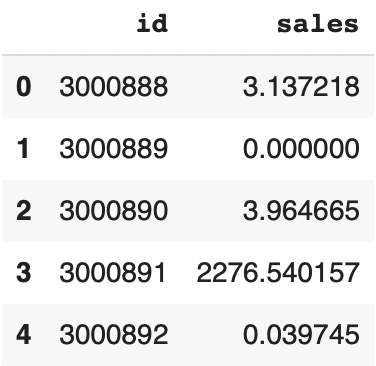

But it’s not over yet! ☝🏻

Now we need to train several models and apply the Ensemble method.

Multiple models

As explained before, the important thing in this code is the hyperparameters. We will train 3 models by taking the following hyperparameters:

model_params = [
    {"lags" : 7, "lags_future_covariates" : (16,1), "lags_past_covariates" : [-16,-17,-18,-19,-20,-21,-22]},
    {"lags" : 365, "lags_future_covariates" : (14,1), "lags_past_covariates" : [-16,-17,-18,-19,-20,-21,-22]},
    {"lags" : 730, "lags_future_covariates" : (14,1), "lags_past_covariates" : [-16,-17,-18,-19,-20,-21,-22]}
]

For each of these parameters, we will train 33 models, run the predictions and fill the final DataFrame. The 3 DataFrames obtained will be stored in the submission_kaggle_list :

from sklearn.metrics import mean_squared_log_error as msle, mean_squared_error as mse
from lightgbm import early_stopping

submission_kaggle_list = []

for params in model_params:

  LGBM_Models_Submission = {}

  display("Training...")

  for family in tqdm(family_list):

    # Define Data for family
    sales_family = family_TS_transformed_dict[family]
    training_data = [ts for ts in sales_family] 
    TCN_covariates = future_covariates_dict[family]
    train_sliced = [training_data[i].slice_intersect(TCN_covariates[i]) for i in range(0,len(training_data))]

    LGBM_Model_Submission = LightGBMModel(lags = params["lags"],
                                          lags_future_covariates = params["lags_future_covariates"],
                                          lags_past_covariates = params["lags_past_covariates"],
                                          output_chunk_length=1,
                                          random_state=2022,
                                          gpu_use_dp= "false")
      
    LGBM_Model_Submission.fit(series=train_sliced, 
                          future_covariates=TCN_covariates,
                          past_covariates=transactions_transformed)

    LGBM_Models_Submission[family] = LGBM_Model_Submission
    
  display("Predictions...")


  LGBM_Forecasts_Families_Submission = {}

  for family in tqdm(family_list):

    sales_family = family_TS_transformed_dict[family]
    training_data = [ts for ts in sales_family]
    LGBM_covariates = future_covariates_dict[family]
    train_sliced = [training_data[i].slice_intersect(TCN_covariates[i]) for i in range(0,len(training_data))]

    forecast_LGBM = LGBM_Models_Submission[family].predict(n=16,
                                          series=train_sliced,
                                          future_covariates=LGBM_covariates,
                                          past_covariates=transactions_transformed)
    
    LGBM_Forecasts_Families_Submission[family] = forecast_LGBM

  # Transform Back

  LGBM_Forecasts_Families_back_Submission = {}

  for family in tqdm(family_list):

    LGBM_Forecasts_Families_back_Submission[family] = family_pipeline_dict[family].inverse_transform(LGBM_Forecasts_Families_Submission[family], partial=True)

  # Prepare Submission in Correct Format

  for family in tqdm(LGBM_Forecasts_Families_back_Submission):
    for n in range(0,len(LGBM_Forecasts_Families_back_Submission[family])):
      if (family_TS_dict[family][n].univariate_values()[-21:] == 0).all():
          LGBM_Forecasts_Families_back_Submission[family][n] = LGBM_Forecasts_Families_back_Submission[family][n].map(lambda x: x * 0)
          
  listofseries = []

  for store in tqdm(range(0,54)):
    for family in family_list:
        oneforecast = LGBM_Forecasts_Families_back_Submission[family][store].pd_dataframe()
        oneforecast.columns = ['fcast']
        listofseries.append(oneforecast)

  df_forecasts = pd.concat(listofseries) 
  df_forecasts.reset_index(drop=True, inplace=True)

  # No Negative Forecasts
  df_forecasts[df_forecasts < 0] = 0
  forecasts_kaggle = pd.concat([df_test_sorted, df_forecasts.set_index(df_test_sorted.index)], axis=1)
  forecasts_kaggle_sorted = forecasts_kaggle.sort_values(by=['id'])
  forecasts_kaggle_sorted = forecasts_kaggle_sorted.drop(['date','store_nbr','family'], axis=1)
  forecasts_kaggle_sorted = forecasts_kaggle_sorted.rename(columns={"fcast": "sales"})
  forecasts_kaggle_sorted = forecasts_kaggle_sorted.reset_index(drop=True)

  # Submission
  submission_kaggle_list.append(forecasts_kaggle_sorted)

We end up with four prediction DataFrames that we will sum and average (this is the so-called ensemble method):

df_sample_submission['sales'] = (submission_kaggle[['sales']]+submission_kaggle_list[0][['sales']]+submission_kaggle_list[1][['sales']]+submission_kaggle_list[2][['sales']])/4

Here is the result:

df_sample_submission.head()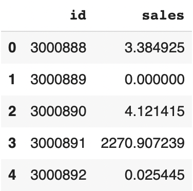

You can now save the predictions in a CSV file and submit it to Kaggle:

df_sample_submission.to_csv('submission.csv', index=False)

Feel free to tweak the hyperparameters to improve the model.

If you liked this tutorial, you can put a like on my Kaggle notebook, it will help me a lot !

See you soon on Inside Machine Learning! 😉

top 1 kaggle top 1 kaggle top 1 kaggle top 1 kaggle top 1 kaggle top 1 kaggle top 1 kaggle top 1 kaggle top 1 kaggle