Ensemble Methods – Everything you need to know now

In this tutorial, we will see how to use Ensemble methods, a technique to improve your Deep Learning models precision.

The concept of Ensemble is simple: gather predictions of several Machine Learning Algorithms to obtain an optimal result.

For example, by averaging a Decision Tree and a Linear Regression to get a new result.

The idea is to take several models that each have their qualities and flaws. Then use them together (ensemble) to balance their biases and get a better prediction.

Let’s take a metaphor: imagine you have to mount a piece of Ikea furniture.

You know how to drive nails into wood but screws are not your thing.

You’ll go much faster if you call your screwdriver expert friend.

Ensemble methods are based on the same principle.

Every Machine Learning model has biases.

If you use a new algorithm and combine it with the old one, you can correct these biases and get a better result.

And it works!

Nowadays most of the Machine Learning competitions winners use Ensemble to create the best algorithms.

In this article, I propose you to see the main methods in theory AND in practice using the Scikit-Learn library.

Our dataset

We’ll use the same dataset as in our article to learn Machine Learning with sklearn.

No worries if you didn’t read the article.

You can still follow this tutorial without any problem 😉

First of all, load my Git folder which lists the interesting datasets of ML:

!git clone https://github.com/tkeldenich/datasets.git

We choose the winequality-white.csv dataset and import it into a Pandas DataFrame :

import pandas as pd

df = pd.read_csv("/content/datasets/winequality-white.csv", sep=";")
df.head(3)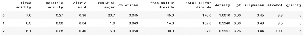

Here a row represents a wine.

Each column is a feature of this wine.

The goal is to predict the wine quality by using its features.

If you want a detailed Data Analysis, I refer you to this article.

It is a classification problem with 7 classes (the wine quality ranging from 3 to 9).

We separate our dataset between the features X and the label Y:

df_features = df.drop(columns='quality')
df_label = df['quality']

Then between the training data and the test data:

from sklearn.model_selection import train_test_split

X_train, X_test, y_train, y_test = train_test_split(df_features, df_label, test_size=0.20)

Done! We are ready to use Ensemble’s methods.

Our goal is to do better than previous Machine Learning algo’s!

Most of them hardly reach an accuracy of 45%.

But the Decision Tree outperforms them all, with an accuracy of 60%.

Let’s try to do better with Ensembles!

Bagging Algorithms

Bagging algorithms use several Machine Learning algorithms called Weak Learners.

They are trained independently on the dataset. This is called parallel training.

Once trained, we gather their results into final predictions.

In order to do this we use, most often, the calculation of the average of the predictions.

Let’s see the different Bagging algorithms that sklearn offers.

Bagging Classifier

Theory

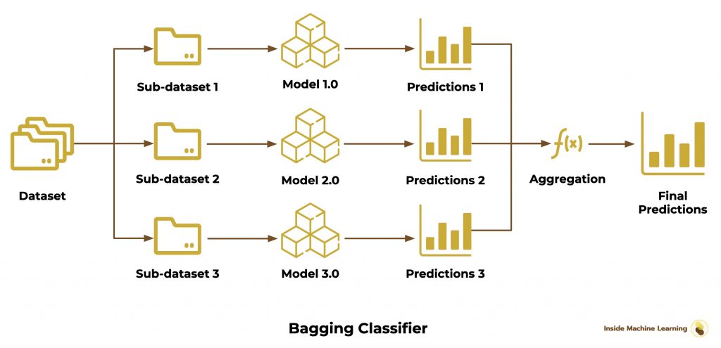
First we have the Bagging Classifier. It is an ensemble of similar algorithms.

Each are trained on a sub-dataset.

The idea is to randomly separate the dataset into several sub-datasets, for example 3.

Each of these 3 sub-datasets will enable to train an algorithm.

At the end, we will have 3 algorithms, trained on different datasets.

I insist on the fact that these algorithms are similar.

That is to say that if you choose a Decision Tree, the 3 algorithms will be Decision Trees with the same hyperparameters baseline.

The only difference is the data they are trained with.

To use this set on new X_test data, we run the 3 algorithms.

We will have 3 results:

• y_pred_1
• y_pred_2
• y_pred_3

The final result is obtained by “aggregating” these results, either by calculating the average of the 3, or by taking the majority choice (this is called “a vote”).

Here is the scheme of the Bagging algorithm:

Understanding the average

Let’s take the first wine. Imagine that we have the following probabilistic results for the 3 algorithms:

1. probability of being of quality 3 = 30% – probability of being of quality 4 = 70%
2. probability of being of quality 3 = 80% – probability of being of quality 4 = 20%
3. probability of being of quality 3 = 70% – probability of being quality 4 = 30%

The average gives us :

probability of being of quality 3 = (30 + 80 + 70) / 3 = 60%

probability of being of quality 4 = (70 + 20 + 30) / 3 = 40%

The Ensemble predicts that the wine is of quality 3!

Understanding the vote

Let’s take the first wine again. But this time we will NOT take the probabilistic results.

We take the direct results of the algorithms. That is, we take the highest probability and assign it a 1. We assign a 0 to the other probabilities.

Here is what it gives us for the 3 algorithms:

1. result for quality 3 = 0 – result for quality 4 = 1
2. result for quality 3 = 1 – result for quality 4 = 0
3. result for quality 3 = 1 – result for quality 4 = 0

Here we look at the quality of wine that has the most 1’s.

Quality 3 wins!

The Ensemble, here also, predicts that the wine is of quality 3.

Practice

The Bagging classifier can seem complicated.

Sklearn makes it super simple!

Here is the code to initialize a Bagging Classifier and train it on our data:

from sklearn.ensemble import BaggingClassifier

baggingClassifier = BaggingClassifier(n_estimators=100)
baggingClassifier.fit(X_train, y_train)

You can see that we don’t need to separate our dataset.

Sklearn takes care of everything.

We can indicate the model on which the Ensemble should be based. But by default, if we don’t indicate anything, sklearn will take a Decision Tree.

We display the result:

baggingClassifier.score(X_test, y_test)

Output: 0.679

We obtain an accuracy of 67.9% ! This is 7.9% more than a classical Decision Tree.

This is a considerable improvement!

Voting Classifier

Theory

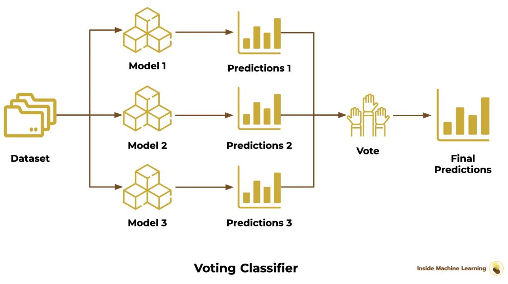
Here we have the Voting Classifier.

It is very similar to the Bagging Classifier.

But it is different.

Here, the Ensemble is not necessarily composed of similar algorithms.

We can have a Decision Tree and two Linear Regression.

Then, the dataset isn’t separated in a random way.

We keep the complete dataset and we train all the models with it.

Finally, we make a vote between algorithms, as we have seen before.

Here is the diagram of the Voting Classifier:

The Voting Classifier is the lengthiest Bagging Ensemble to set up.

We have to choose each model of our ensemble.

We can also add weights to control the importance of each model.

Here I choose to assign the most important weight to the Decision Tree, the best model to solve our problem:

from sklearn.ensemble import VotingClassifier
from sklearn import tree
from sklearn.naive_bayes import GaussianNB
from sklearn.linear_model import SGDClassifier
from sklearn.linear_model import LogisticRegression


decisionTree = tree.DecisionTreeClassifier()
logisticRegression = LogisticRegression()
SGD = SGDClassifier()
GNB = GaussianNB()

votingClassifier = VotingClassifier(estimators=[
    ('tree', decisionTree), ('lr',logisticRegression), ('sgd', SGD), ('gnb', GNB)],
    weights=[2,1,1,0.5])
votingClassifier.fit(X_train, y_train)

Then we compute the Ensemble score:

votingClassifier.score(X_test, y_test)

Output: 0.603

60% accuracy. The Voting Classifier did not give the best result.

Let’s go on to the next step !

Random Forest

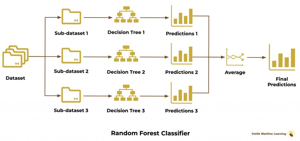
We arrive at the famous Random Forest.

Here, we are expected to break the record!

The Random Forest is a Decision Tree Ensemble (the best model for our project).

As for the Bagging Classifier, we randomly separate our dataset into sub-datasets.

Then we train different Decision Trees on each sub-dataset.

Finally we use the average to obtain the final predictions:

The implementation is very simple with sklearn :

from sklearn.ensemble import RandomForestClassifier

randomForest = RandomForestClassifier(n_estimators=100)
randomForest.fit(X_train, y_train)

Then we compute the score :

randomForest.score(X_test, y_test)

Output: 0.7

70%, our best score! 🔥

We managed to get a good score even though we started with very little advantage on our side.

The first trained model had an accuracy of 46%.

With motivation and the right techniques, we managed to increase this accuracy by more than 24%. That’s huge!

If you’ve been following the project from the beginning until now, you can congratulate yourself!

Let’s continue with the rest of the Ensemble algorithms.

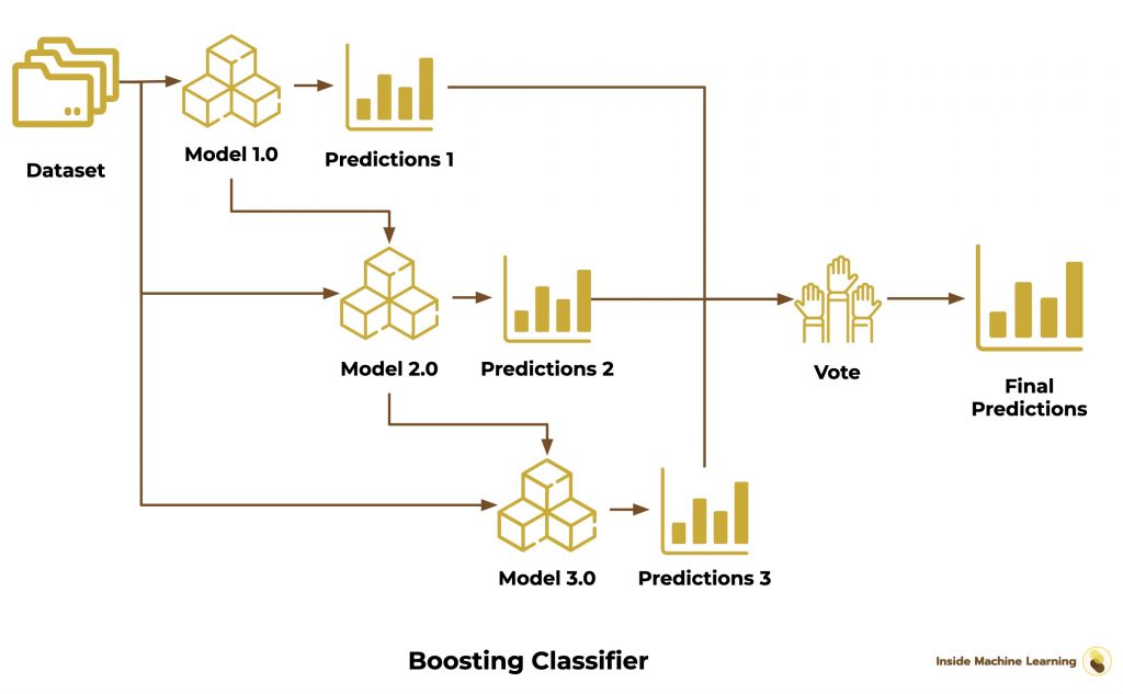
Boosting Algorithm

Boosting algorithms bring together several versions of the same Machine Learning algorithm (Weak Learners).

The first version of the model is trained on the dataset.

Then we create a second version of the model and we also train it on the dataset.

The goal here is to improve the new model version by targeting the weaknesses of the first one.

Each trained algorithm is a new version of the previous one. This is called sequential training.

Finally, as for the Bagging algorithms, we gather the results into final predictions by calculating the average of the predictions.

Let’s go on to the algorithms proposed by sklearn !

AdaBoost

AdaBoost is short for Adaptive Boosting.

The idea is very similar to the Bagging Classifier concept.

We will create several versions of the model.

However, here we do not train it on different sub-datasets.

We train the first model on the whole dataset.

Then we observe its predictions.

We create a new version of the model by adjusting the weights at the level of the incorrect predictions of the first one.

We repeat the process until we are satisfied.

In this way the new model versions focus more on the difficult cases identified by the previous ones.

Thus each model balances the flaws of the others.

The final prediction is a vote or an average of all the models.

Here is the Boosting Classifier scheme:

We use AdaBoost with sklearn like so:

from sklearn.ensemble import AdaBoostClassifier

adaBoost = AdaBoostClassifier(n_estimators=100)
adaBoost.fit(X_train, y_train)

We compute the score :

adaBoost.score(X_test, y_test)

Output: 0.443

We get an accuracy of 44.3%.

For the moment AdaBoost gives us the worst score among the Ensemble methods.

Actually, AdaBoost is THE first Boosting algorithm created.

Today, new Boosting algorithms exist, notably available via the LightGBM, XGBoost or CatBoost libraries.

Gradient Boosting

Historically, AdaBoost is the first boosting algorithm.

Gradient Boosting follows it closely.

As a matter of fact AdaBoost allows to solve specific problems.

Seeing its promising results, researchers decided to generalize the mathematical approach of AdaBoost with the Gradient Boosting algorithm.

Thus Gradient Boosting can solve many more problems than AdaBoost.

And even if AdaBoost is the oldest, it is now seen as a special case of Gradient Boosting.

I don’t want to dive into the mathematical details of the algorithm.

Just keep in mind that GradBoost is a generalization of AdaBoost.

That is, it is efficient on most datasets, unlike AdaBoost which is more specific.

And if you are a curious mathematician, here are the resources that will interest you:

• Invent Adaboost, the first successful boosting algorithm [Freund et al., 1996, Freund and Schapire, 1997]
• Formulate Adaboost as gradient descent with a special loss function[Breiman et al., 1998, Breiman, 1999]
• Generalize Adaboost to Gradient Boosting in order to handle a variety of loss functions [Friedman et al., 2000, Friedman, 2001]

The scheme of Gradient Boosting is the same as AdaBoost since only the underlying mathematics is different.

Here is how to use Gradient Boosting with sklearn:

from sklearn.ensemble import GradientBoostingClassifier

gradientBoosting = GradientBoostingClassifier(n_estimators=100, learning_rate=1.0,max_depth=1, random_state=0)
gradientBoosting.fit(X_train, y_train)

We compute the score:

gradientBoosting.score(X_test, y_test)

Output: 0.524

52% accuracy, the improvement over AdaBoost is noticeable.

But let’s see an even more recent evolution of Gradient Boosting.

Histogram-Based Gradient Boosting

To put it simply, Histogram-Based Gradient Boosting is a faster version of GradBoost.

Faster and therefore easier to calculate.

It allows to allocate more time to the optimization. And thus to obtain better results.

Histogram-Based Gradient Boosting uses a data structure called histogram in which the elements are implicitly ordered.

This enables a fast processing of the information.

Again, you can refer to the AdaBoost scheme as the only difference is mathematical.

Here is how to use Histogram-Based Gradient Boosting:

from sklearn.ensemble import HistGradientBoostingClassifier

histGradientBoostingClassifier = HistGradientBoostingClassifier(max_iter=100)
histGradientBoostingClassifier.fit(X_train, y_train)

Then we compute the score :

histGradientBoostingClassifier.score(X_test, y_test)

Output: 0.671

67.1% accuracy. Congratulations!

That is the best score for Boosting algorithms!

We can finally move on to the last types of Ensemble algorithms…

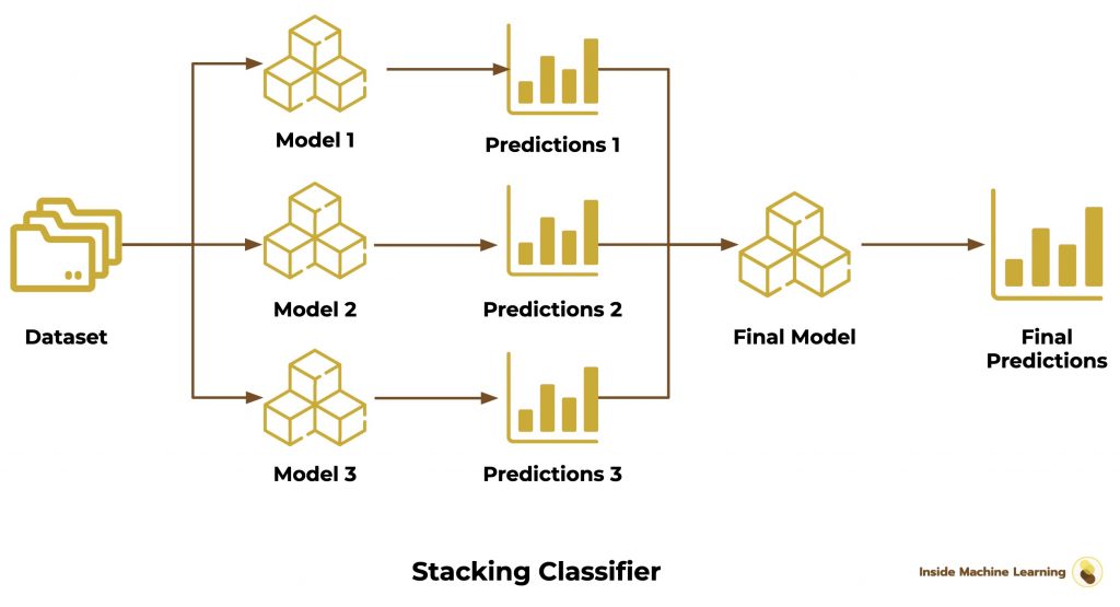
Stacking algorithms

Stacking algorithms use the results of several Machine Learning algorithms. These results are then used as input for a final algorithm that gives the prediction.

The algorithms are trained independently on the dataset.

As with Bagging, it is a parallel training.

The predictions are then gathered (stacked).

A last algorithm is finally used on all the results to obtain the final predictions.

Sklearn offers us a single Stacking algorithm:

Stacking Classifier

The Stacking Classifier works according to the classical Stacking method.

On top of that, the final model is trained using cross-validation, a technique we’ve already discussed in this article.

Here is the scheme of the Stacking Classifier:

To use it, we specify the models we want to use:

• the models to be trained in parallel
• the final prediction model

from sklearn.ensemble import StackingClassifier
from sklearn import tree
from sklearn.naive_bayes import GaussianNB
from sklearn.linear_model import SGDClassifier
from sklearn.linear_model import LogisticRegression


decisionTree = tree.DecisionTreeClassifier()
logisticRegression = LogisticRegression()
SGD = SGDClassifier()
GNB = GaussianNB()
finalClassifier = LogisticRegression()

stackingClassifier = StackingClassifier(estimators=[
    ('tree', decisionTree), ('lr',logisticRegression), ('sgd', SGD), ('gnb', GNB)],
    final_estimator=finalClassifier)
stackingClassifier.fit(X_train, y_train)

And we compute the score:

stackingClassifier.score(X_test, y_test)

Output: 0.477

For this last method, we obtain an accuracy of 47.7% !

Conclusion

The Random Forest is undoubtedly the best Ensemble method to use for our dataset with 70% accuracy!

It is closely followed by the Bagging Classifier and the Histogram-Based Gradient Boosting which both give us 67% accuracy.

Here is what you should remember about the 3 types of Ensemble algorithms:

	Learning	Technique	Advantage
Bagging	Parallel	Assembly of different models	Diversified approach
Boosting	Sequential	Assembly of several versions of the same model	Successive Improvement
Stacking	Parallel + Stacked	Assembly of different models evaluated by a final model	Assembly evaluated by an Independent model

This is the end of this extensive article on Ensemble methods.

If you’ve made it this far, you’ve accumulated a lot of information.

In the future, you can refer to the schemes that provide a solid foundation for understanding Ensemble methods.

Use them!

There is a reason why they’re the favorites in Machine Learning competitions.

With them, your models will reach the next level.

And if you are looking for other techniques to improve your Machine Learning algorithms,follow this way:

• Normalize data
• Cross-Validation
• Changing the models hyperparameters
• Data Augmentation

See you soon on Inside Machine Learning 😉

sources :

• Scikit-learn Documentation – Ensemble methods
• Cheng Li, Northeastern University – A Gentle Introduction to Gradient Boosting
• StackExchange – Intuitive explanations of differences between Gradient Boosting Trees (GBM) & Adaboost
• StackExchange – Adaboost vs Gradient Boosting
• Medium – Ensemble methods: bagging, boosting and stacking