

Normalize your data in 3 easy ways, both for DataFrame and Numpy Array. This is the challenge of this article!
Normalization is changing the scale of the values in a dataset to standardize them.
Instead of having a column of data going from 8 to 1800 and another one going from -37 to 90, we normalize the whole to make them go from 0 to 1.
But why normalize?
By normalizing each of our columns so that they have the same distribution, we help our Machine Learning model during its learning process. Indeed, this allows the model to analyze each of our columns using the same approach.
Thus the model does not have to adapt its input channels to different scales but only to one.
In mathematical language: normalization helps optimize the loss function and make it converge faster.
This makes it a technique used for both Machine Learning and Deep Learning.
The larger the number of columns in a dataset, the longer it takes to manually normalize it.
Fortunately for us, Scikit-Learn allows us to perform this task automatically.
Let’s see that right now!
Data
For this tutorial we will use the wine quality dataset.
We used it in this detailed article to learn Machine Learning.
The objective is to predict the quality of wine from its features (acidity, alcohol content, pH, etc). You can download the dataset from this Github address.
Once loaded in your work environment, open it with the Pandas library:
import pandas as pd

df = pd.read_csv("winequality-white.csv", sep=";")
df.head(3)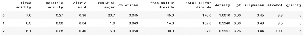
We separate the label (the quality level of the wine) from the features (characteristics that will help us predict the label):
df_features = df.drop(columns='quality')
df_label = df['quality']
And we can start the normalization.
As explained before, normalization is changing the scale of values of the columns of our dataset.
But what defines this scale?
Let’s take the fixed acidity column, the scale is first determined by the minimum and maximum value.
Minimum and maximum are the values between which all the others oscillate.
Then we have the mean: the sum of these data divided by their total number.
And the standard deviation, which measures how far the values in the dataset are from the mean. The higher the value of standard deviation, the further the values are from the mean.
Let’s display these measurements for the fixed acidity column.
print(f'Min : ',df_features['fixed acidity'].min(),', Max :', df_features['fixed acidity'].max())
print(f'Mean : ',round(df_features['fixed acidity'].mean(),2),', Standard Deviation :', round(df_features['fixed acidity'].std(),2))
Output :
Min : 3.8 , Max : 14.2
Mean : 6.85 , Standard Deviation : 0.84
Other metric exist to measure the scale of a dataset but these are the main ones.
Normalization is modify these measures (while preserving the information), thanks to mathematical functions, to include them in the scale of our choice.
Normalization between 0 and 1
One of the most basic normalizations is the 0 to 1 normalization.
We modify our data so that they fall in the interval in the interval [0, 1].
The minimum will be 0 and the maximum will be 1.
For this we initialize MinMaxScaler() of the preprocessing package of sklearn :
from sklearn import preprocessing

transformer = preprocessing.MinMaxScaler().fit(df_features[['fixed acidity']])
Then we use the transform() function on our fixed acidity column to normalize it:
X_transformed = transformer.transform(df_features[['fixed acidity']])You can display X_transformed and see that the values have been transformed. They have been normalized.
This does not or hardly degrade our data.
Indeed, the normalization modifies the value of the data but does so while preserving the information about the distance between each point.
Moreover, it suffices to use the inverse_transform() function to return to the previous values.
Be aware that the transformation converts your DataFrame into a Numpy Array. To have a DataFrame instead of a Numpy Array, use after the normalization operation : df = pd.DataFrame(X_transformed, columns = ['fixed acidity', 'volatile acidity', 'citric acid', 'residual sugar', 'chlorides', 'free sulfur dioxide', 'total sulfur dioxide', 'density', 'pH', 'sulphates', 'alcohol']).
The measurements can now be displayed to confirm that normalization has occurred:
By the way, if your goal is to master Deep Learning - I've prepared the Action plan to Master Neural networks. for you.
7 days of free advice from an Artificial Intelligence engineer to learn how to master neural networks from scratch:
- Plan your training
- Structure your projects
- Develop your Artificial Intelligence algorithms
I have based this program on scientific facts, on approaches proven by researchers, but also on my own techniques, which I have devised as I have gained experience in the field of Deep Learning.
To access it, click here :
Now we can get back to what I was talking about earlier.
print(f'Min : ',round(X_transformed.min(),2),', Max :', round(X_transformed.max(),2))
print(f'Mean : ',round(X_transformed.mean(),2),', Standard Deviation :', round(X_transformed.std(),2))
Output :
Min : 0.0 , Max : 1.0
Mean : 0.29 , Standard Deviation : 0.08
Normalization between -1 and 1
Another usual normalization is the normalization from -1 to 1.
We use the same function as before MinMaxScaler() but, here, we indicate the feature_range attribute which determines the normalization interval: (-1, 1)
from sklearn import preprocessing

transformer2 = preprocessing.MinMaxScaler(feature_range=(-1, 1)).fit(df_features[['fixed acidity']])
We apply the transformation :
X_transformed2 = transformer2.transform(df_features[['fixed acidity']])And we display the measurements:
print(f'Min : ',round(X_transformed2.min(),2),', Max :', round(X_transformed2.max(),2))
print(f'Mean : ',round(X_transformed2.mean(),2),', Standard Deviation :', round(X_transformed2.std(),2))
Output :
Min : -1.0 , Max : 1.0
Mean : -0.41 , Standard Deviation : 0.16
Note that the function can be used for any type of interval (-10, 10), (-100, 100), etc.
Obtaining a Normal Distribution (Normal Law)
Let’s move on to a normalization more prized by experts.
Normal Law normalization, also called standardization, consists in modifying the scale of a data set in such a way as to obtain :
- A standard deviation of 1
- A mean of 0
Standardization is ideal when we have outliers, data that are unusually far from the mean.
Indeed, in the previous standardizations, we imposed a limit to our data: between 0 and 1 for example.
With standardization, there is no limit, only the requirement to have a mean of 0 and a standard deviation of 1.
Thus, when the dataset has outliers, it is preferable to use standardization. The non-limitation offered by standardization allows us to preserve the information about the unusual distance of the outliers.
To standardize we use StandardScaler:
from sklearn import preprocessing

transformer = preprocessing.StandardScaler().fit(df_features[['fixed acidity']])
We apply the transformation :
X_transformed3 = transformer.transform(df_features[['fixed acidity']])And we display the measurements:
print(f'Min : ',round(X_transformed3.min(),2),', Max :', round(X_transformed3.max(),2))
print(f'Mean : ',round(X_transformed3.mean(),2),', Standard Deviation :', round(X_transformed3.std(),2))
Output :
Min : -3.62 , Max : 15.03
Mean : 0.0 , Standard Deviation : 1.0
The Power of Normalization
Is great to know how to use normalization, but does it work?
In our detailed article on how to learn Machine Learning we explored several models to determine the most efficient.
Result: the best model was the Decision Tree with an accuracy of 60%.
A satisfactory score considering the correlation between our features and the label but…
… can we improve this score with normalization ?
Let’s see that now ! 🔥
Here we initialize the standardization on all our features:
from sklearn import preprocessing

transformer = preprocessing.StandardScaler().fit(df_features)
We apply the transformation :
df_features_transformed = transformer.transform(df_features)Now we can separate our data for training and testing:
from sklearn.model_selection import train_test_split

X_train, X_test, y_train, y_test = train_test_split(df_features, df_label, test_size=0.20)
Now let’s train our Decision Tree:
from sklearn import tree

decisionTree = tree.DecisionTreeClassifier()
decisionTree.fit(X_train, y_train)
Finally let’s compute its accuracy:
decisionTree.score(X_test, y_test)Output:
0.626
62.6% of accuracy!
With normalization we managed to increase the performance of the model by 2.6%.
This may not seem much to the eyes of a beginner, but experts know that increasing the accuracy of a model by even 1% is already tremendous.
And you, what score did you achieve with normalization?
There are many other methods to improve a Machine Learning model. After normalization, we can mention :
See you soon in a next article!
And if you want to stay informed don’t hesitate to subscribe to our newsletter 😉
One last word, if you want to go further and learn about Deep Learning - I've prepared for you the Action plan to Master Neural networks. for you.
7 days of free advice from an Artificial Intelligence engineer to learn how to master neural networks from scratch:
- Plan your training
- Structure your projects
- Develop your Artificial Intelligence algorithms
I have based this program on scientific facts, on approaches proven by researchers, but also on my own techniques, which I have devised as I have gained experience in the field of Deep Learning.
To access it, click here :