Binary Classification NLP – Best simple and efficient model

In this article, we’ll look at the classic approach to use in order to perform Binary Classification in NLP.

Binary classification is a two-option classification problem.

For this NLP binary classification we use a dataset available in the Keras library.

This dataset is composed of :

• movie reviews
• labels (0 or 1) associated to each review

The labels indicate if the review is positive (1) or negative (0).

The goal of our Deep Learning model will be to determine from a movie review whether the viewer liked the movie or not, i.e. whether the review is positive or not. There are only two possible options, this is called a binary classification.

So we will train our model on training data and then test it, check its capabilities on test data.

[smartslider3 slider=”15″]

Photo by Konstantin Kleine on Unsplash

Prepare our data – Binary Classification NLP

Load our data

First, we load the data from the imdb package.

train_data and train_labels are the data on which we will train our model.

There are 50 000 reviews and therefore 50 000 labels. We train our model to predict the labels from the reviews.

Then we can test the efficiency of the model by making predictions on the test_data and by comparing these label predictions to the real label test_labels.

from keras.datasets import imdb

(train_data, train_labels), (test_data, test_labels) = imdb.load_data(num_words=10000)

The movie reviews (stored in train_data and test_data) have already been preprocessed.

That is, the reviews have been transformed, encoded into numbers.

Thus, a sentence is represented by a list of numbers.

Each number represents a word.

num_words=10000 means that we have kept the 10 000 most frequent words in all the reviews.

So we have an index list of 10 000 words and each number in the reviews refers to one of the words in this index list.

If a sentence contains the word number 15, to know it you have to look for the number 15 of the list of 10 000 words.

You can check this by displaying the first review :

print(train_data[0])

[1, 14, 22, …, 19, 178, 32]

Verify our data

We can also translate, decode these reviews to read them in English.

To do this, we load the word_index, a dictionary that contains 88 584 words (the 10,000 most frequent words we have loaded are taken from this dictionary).

word_index = imdb.get_word_index()

This dictionary contains 88 584 words and an index/number for each word.

If we take our previous example to decode the number 15, we must look in the word_index for the corresponding word to the number 15.

We can display the first 5 words of the dictionary:

list(word_index.items())[:5]

We obtain: [(‘fawn’, 34701), (‘tsukino’, 52006), (‘nunnery’, 52007), (‘sonja’, 16816), (‘vani’, 63951)]

For more convenience and speed in decoding we will reverse the dictionary to have the index on the left and the word on the right.

reverse_word_index = dict([(value, key) for (key, value) in word_index.items()])

Display again the first 5 words to see the change:

list(reverse_word_index.items())[:5]

[(34701, ‘fawn’), (52006, ‘tsukino’), (52007, ‘nunnery’), (16816, ‘sonja’), (63951, ‘vani’)]

We can then decode the reviews.

Here, for each number in a review we look at its index in the dictionary.

We get the words associated with the indexes.

Then we join each of these words to make a sentence.

decoded_review = ' '.join([reverse_word_index.get(i - 3, '?') for i in train_data[0]])

print(decoded_review)

The review decoded : “this film was just brilliant casting location scenery story direction everyone’s really suited…”

You can also see the associated label. The review is :

• positive if the label is 1
• negative if the label is 0

print(train_labels[0])

Preprocessing: One-hot encoding – Binary Classification NLP

Although the reviews are already digitally encoded, we need to do a second processing, a second encoding.

We will do what is called a hot-one encoding.
This is a very common encoding in NLP, in word processing.

The hot-one encoding consists in taking into account all the words we are interested in (the 10 000 most frequent words). Each review will be a list of length 10 000 and if a word appears in the review it is encoded as 1 otherwise as 0.

For example, encoding the sequence [3, 5] will give us a vector of length 10 000 which will be made of 0 except for the indices 3 and 5, which will be 1.

This will allow the model to learn quicker and easier.

So we will code the vectorize_sequences function to encode in one-hot :

import numpy as np

def vectorize_sequences(sequences, dimension=10000):
 results = np.zeros((len(sequences), dimension))
 for i, sequence in enumerate(sequences):
  results[i, sequence] = 1.
 return results

x_train = vectorize_sequences(train_data)
x_test = vectorize_sequences(test_data)

We can then display the first element of the x_train to check the one-hot encoding.

print(x_train[0])

[0. 1. 1. ... 0. 0. 0.]

Here we change the type of the labels to float32 instead of int64 (our x_train and x_test are also in float format).

y_train = np.asarray(train_labels).astype('float32')
y_test = np.asarray(test_labels).astype('float32')

Create our Deep Learning model – Binary Classification NLP

Structuring

For this classification we have a very simple data configuration:

• input data in a list of 1 and 0
• data to be predicted 1 or 0
  

The type of network useful in this case is a Dense layer stack, which is still called fully-connected layers, because all neurons are connected to all previous ones. They are fully connected (see this article for more information on neurons).

However, different activation functions are used.

• relu for the first two
• sigmoid for the last one

A whole article will be written about these activation functions. For the moment it is enough to know that the sigmoid function allows to have a probability between 0 and 1.

So the closer the result will be to 1 the more positive the criticism will be and vice versa.

from keras import models
from keras import layers

model = models.Sequential()
model.add(layers.Dense(16, activation='relu', input_shape=(10000,)))
model.add(layers.Dense(16, activation='relu'))
model.add(layers.Dense(1, activation='sigmoid'))

To understand what is happening in this model, we can look at the associated diagram with the plot_model() function.

We can see the change of dimension on our data by looking at the right part of each layer.

Thus, we start with a list of 10 000 words (one-hot encoded) thus a list of length 10 000.

Then the first Dense layer applies a transformation and produces a list of length 16.

Second layer also applies a transformation to produce a list of length 16.

And finally, the last layer applies a transformation that produces a probability between 0 and 1, so a single number, a single dimension.

from keras.utils.vis_utils import plot_model

plot_model(model, to_file='model_plot.png', show_shapes=True, show_layer_names=True)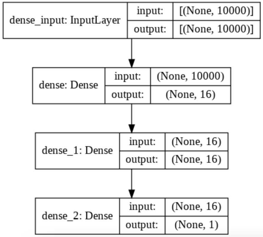

Training

Last preparation before using the model.

These data must be separated into two types :

• training data will be used to train the model
• validation data will validate its learning

In fact, this avoids a frequent problem in Machine Learning: overfitting.

Overfitting is when a model becomes so specialized on its training data that it becomes inefficient on other data, real data. This phenomenon is also called overlearning.

It’s like practicing tennis every day but only on your backhand. In a real match you will perform on your backhand but your forehand will not be that good.

The idea is to train our model well on general data and not to overtrain it.

x_train is composed of 25 000 lists, each of length 10 000.

We separate this data as follows:

• 15 000 lists for training data
• 10 000 lists for the validation data

x_val = x_train[:10000]
partial_x_train = x_train[10000:]

y_val = y_train[:10000]
partial_y_train = y_train[10000:]

We can then compile the model by choosing the optimizer, the loss function and the metric.

Afterwards we can train the model with the fit() function.

The history variable allows us to keep the history of the training.

model.compile(optimizer='rmsprop',
              loss='binary_crossentropy',
              metrics=['accuracy'])

history = model.fit(partial_x_train,
                    partial_y_train,
                    epochs=20,
                    batch_size=512,
                    validation_data=(x_val, y_val))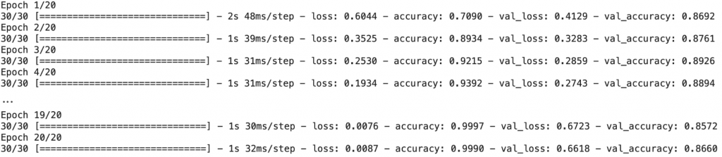

Evaluate

In the history variable we have the values of loss and accuracy.

history_dict = history.history
history_dict.keys()

We will plot a graph with these values to analyze the learning of our model.

import matplotlib.pyplot as plt

history_dict = history.history

loss_values = history_dict['loss']
val_loss_values = history_dict['val_loss']

epochs = range(1, len(loss_values) + 1)

plt.plot(epochs, loss_values, 'bo', label='Training loss')
plt.plot(epochs, val_loss_values, 'b', label='Validation loss')

plt.title('Training and validation loss')
plt.xlabel('Epochs')
plt.ylabel('Loss')
plt.legend()
plt.show()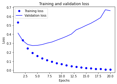

We see at the first epochs that the loss on the training data and the loss on the validation data decrease in a similar way.

Very quickly the curves do not decrease as fast (which is normal) and at one point, at epoch 4, the loss on the validation data increases and does not decrease anymore.

This is exactly where the overfitting is.

The model specializes on the training data so the loss only decreases for these data but by specializing so much it is no longer able to perform on the validation data and, in general, on the real data.

We can verify this fact by plotting the accuracy curve of the model on the training data and on the validation data.

Indeed, the accuracy decreases from epoch 4 for the validation data while it continues to increase for the training data.

plt.clf()

acc_values = history_dict['accuracy']
val_acc_values = history_dict['val_accuracy']

plt.plot(epochs, acc_values, 'bo', label='Training accuracy')
plt.plot(epochs, val_acc_values, 'b', label='Validation accuracy')

plt.title('Training and validation accuracy')
plt.xlabel('Epochs')
plt.ylabel('Accuracy')
plt.legend()
plt.show()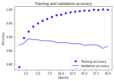

We can also evaluate our model on the test data.

We have on the left the loss and on the right the precision.

Here be careful not to confuse the two metrics:

• precision can be taken as a percentage, if it is 0.85 then 85%.
• loss is not a percentage, our goal is only to make it tend towards 0

model.evaluate(x_test, y_test)

[0.7295163869857788, 0.8501999974250793]

After this analysis, we can improve our model.

Improve

We have seen that the model learns very well on training data but less well on validation data.

Our model reaches its peak performance at epoch 4.

Therefore, we will reduce the number of epochs to improve the performance of our model!

model = models.Sequential()
model.add(layers.Dense(16, activation='relu', input_shape=(10000,)))
model.add(layers.Dense(16, activation='relu'))
model.add(layers.Dense(1, activation='sigmoid'))

model.compile(optimizer='rmsprop',
              loss='binary_crossentropy',
              metrics=['accuracy'])

model.fit(x_train, y_train, epochs=4, batch_size=512)

results = model.evaluate(x_test, y_test)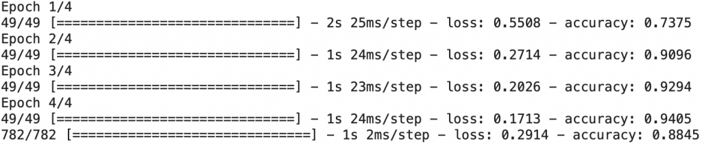

And that’s it! We can evaluate our model again on the test data to see the improvement that occurred on the loss (lower) and on the accuracy (higher).

print(results)

[0.2913535237312317, 0.8844799995422363]

To use the model on new data, nothing could be simpler, you have to use the predict() function.

This will generate the probability that the reviews are positive.

model.predict(x_test[0:2])

The first criticism has a probability of 0.20192459 to be positive, so it is surely negative.

The second criticism has a probability of 0.99917173 to be positive, the model is almost certain that the criticism is positive.

To go further…

Deep Learning is all about practice ! There is no theoretical secret that will allow you to improve the accuracy of a model.

Increasing the performance of your model is a matter of testing, experimenting and tinkering.

Don’t hesitate to add layers of neurons, to change the different hyperparameters to see the changes that this operates on the results of the model.

Here by changing the dimension of the first Dense layer, the loss function, the batch_size and the epochs we get a better performing model !

model = models.Sequential()
model.add(layers.Dense(64, activation='relu', input_shape=(10000,)))
model.add(layers.Dense(16, activation='relu'))
model.add(layers.Dense(1, activation='sigmoid'))

model.compile(optimizer='rmsprop',
              loss='mse',
              metrics=['accuracy'])

model.fit(x_train, y_train, epochs=3, batch_size=256)

results = model.evaluate(x_test, y_test)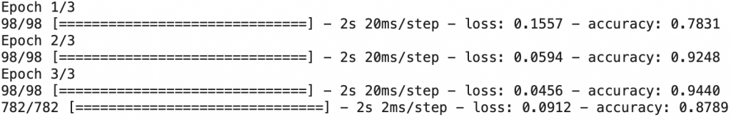

Our NLP Binary Classification model achieves 87% accuracy!

Thanks to our neural network, we’ve created an AI with a high degree of precision.

Deep Learning is a powerful approach! 🚀

This is the reason why Google, Amazon, Meta and OpenAI are using this technology to create the Artificial Intelligences of tomorrow.

If you want to deepen your knowledge in the field, you can access my Action plan to Master Neural networks.

A program of 7 free courses that I’ve prepared to guide you on your journey to learn Deep Learning.

To access it, click here:

GET MY ACTION PLAN