Activation function: How it works – Best Simple Guide

In this article, we’ll take a detailed look at what an activation function is and how it can be used in a Deep Learning model!

Previously, we explored the fundamental concepts of Deep Learning: layer, neuron and weight.

We discovered that a Deep Learning model doesn’t quite work like the human brain.

In fact, this myth, unfortunately widespread, is incorrect.

Information Processing – Human Brain vs. Deep Learning

To predict an event, we humans analyze data, and only then make a prediction.

This is a two-stage approach: analysis-prediction.

For example, if we wanted to try and predict the outcome of a match at Roland Garros, we’d look at the results of previous matches, then project ourselves into the future to try and predict a winner.

You’ll agree that this approach isn’t the most scientific. It doesn’t guarantee us a quality prediction. It’s a flaw in the human brain. It’s not 100% reliable. But it’s the same flaw that allows us to be caught off guard when the Machiavellian Joffrey Baratheon is poisoned at his wedding. It’s a situation that’s hard for our brains to predict… but that’s what makes it so enjoyable. If this little flaw allows us to enjoy Game of Thrones, we won’t complain!

A Deep Learning model employs a different approach. It ingests data and transforms it to produce a result.

To return to the Roland Garros example, a Deep Learning model would not analyze the statistics of previous matches and then make a prediction. Instead, it would take the statistics and apply successive transformations to obtain a result.

A Deep Learning model therefore uses a one-step approach: forward propagation.

Forward propagation is the process of propagating and transforming data through a neural network.

In today’s article, we’ll be looking at one of the key components of forward propagation: the activation function. We’ll explore the theory of activation functions, their application in programming and the underlying mathematical operations.

What is an Activation Function?

The process of forward propagation enables a neural network to produce a result from data.

Before the result is produced, the data passes through the model. Each neuron then receives the data and applies a transformation to it. This succession of transformations produces a result.

The transformation in question is a mathematical operation performed by a neuron using its activation function and weight.

Activation function is the attribute of the neuron enabling it to transform data.

It plays a central role in a neural network, allowing a non-linear transformation to be applied.

Non-linearity is a mathematical concept. If your goal is simply to practice Deep Learning, you won’t need to delve into it. However, understanding its impact is important, as it is the source of the performance of Deep Learning algorithms.

Nonlinearity and Spatial Representation

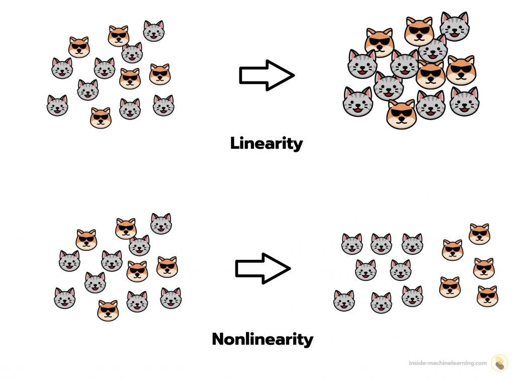
A non-linear transformation modifies the spatial representation of data.

This transformation gives us the ability to explore the data from different perspectives and thus better understand it.

Conversely, a linear transformation may modify the data, but has no influence on its spatial representation.

To illustrate this, let’s imagine we have two values: 13 and 54. These values have a spatial representation: 13 is less than 54. If we apply a linear operation, such as multiplication by 2, the value of these data will change. However, their spatial position will remain unchanged: 13x2 = 26 will always be less than 54x2 = 108.

Linear transformations therefore have no impact on the spatial representation of data. But non-linear transformations do.

If we apply a non-linear operation to 13 and 54, for example the cosine function, this will change the value of the data, but also their spatial position: cos(13) ≈ 0.90 is greater than cos(54) ≈ -0.82.

To refine our understanding of the data, we will then need to use a non-linear transformation.

This property of non-linear functions is a major asset, which is why neural networks exploit it through activation functions. Neural networks can thus extract relevant information from a dataset during forward propagation to produce quality predictions!

Non-linearity is one of the features that differentiates Deep Learning algorithms from traditional Machine Learning algorithms – you can read more about it in this article.

The Role of Activation Functions in Deep Learning Models

As mentioned previously, each neuron has an activation function and a weight. However, while the weights are randomly assigned to all neurons, the activation function is chosen manually by the ML Engineer.

A model can be made up of thousands of neurons, or even more. Consequently, the ML Engineer will not assign an activation function individually to each neuron. That would take a lot of time!

Instead, the activation function is selected by the ML Engineer when adding a layer to the model. The activation function is then automatically distributed to the neurons in that layer.

In this way, neurons in the same layer share the same activation function.

In Practice

With Keras, when you add a Dense layer, you can also specify an activation function:

model.add(layers.Dense(32, activation='sigmoid'))

Here, the activation function chosen is the sigmoid function. It will be associated with the 32 neurons in the layer.

Keras is designed to facilitate Deep Learning, so we can call the sigmoid function with a simple string 'sigmoid'. However, it’s important to note that it can also be called as a :

tf.keras.activations.sigmoid(x)

This practice is generally used in low-level libraries such as TensorFlow and PyTorch, designed for people with in-depth Deep Learning experience. But it can also be done with Keras.

Furthermore, it’s important to emphasize that activation functions are not just attributes of Deep Learning layers. They are also functions, apart from Deep Learning algorithms, that can be used to modify data.

In the context of Deep Learning, there are several activation functions. It’s vital to know what they are and how to select them. Indeed, if you choose the wrong activation function, you could sabotage an entire model. And believe me, you don’t want your neural network to end up like Joffrey Baratheon.

Before moving on to the math-centric section, if you like my pedagogy, you can delve deeper into Deep Learning with me in my private e-mails.

In addition to my monthly newsletter, you can follow my new Action plan to Master Neural networks. If you’d like to find out more – click here:

GET MY ACTION PLAN

The Different Activation Functions

To further clarify this section, when explaining the use of activation functions with Keras, I’ll use the function call.

In mathematics, an uncountable number of non-linear functions exist. Nevertheless, only a small fraction of them are used as activation functions in Deep Learning.

The difference between these activation functions may sometimes seem negligible, but some of them need to be chosen with precision if you want to create a functional neural network.

ReLU

Rectified Linear Unit (ReLU) function is the most commonly used activation function in Deep Learning.

It gives x if x is greater than 0, 0 otherwise. In other words, it’s the maximum between x and 0 :

ReLU_function(x) = max(x, 0)

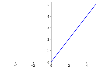
This function applies a filter to the layer output. It allows positive values to pass through to subsequent layers, and blocks negative values. This filter then allows the model to focus only on certain characteristics of the data, while eliminating others.

How to use the ReLU function with Keras :

tf.keras.activations.relu(x, alpha=0.0, max_value=None, threshold=0)

• x: input data, tensor
• max_value: allows to set a maximum value for the outputs of the ReLU function. If max_value is set to a real value, all output values above max_value will be replaced by max_value. This limits the range of function output values
• threshold: defines a threshold for inputs. By default, this threshold is set to 0, meaning that all negative inputs are set to zero. However, this threshold can be modified to suit ML Engineer’s needs.

Sigmoid

Sigmoid function is the activation function used in the last layer of a neural network built to perform a binary classification task.

It gives a value between 0 and 1.

Sigmoid_function(x) = 1 / (1 + exp(-x))

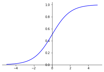
This value can be interpreted as a probability. In a binary classification, the sigmoid activation function can then be used to obtain, for a given item, the probability of belonging to a class.

I used it notably in my project for classifying movie reviews. In this example, the closer the sigmoid result is to 1, the more the model considers the review to be positive. Conversely, the closer the sigmoid result is to 0, the more the model considers the review to be negative.

The sigmoid activation function therefore provides an ambivalent result, giving an indication of two classes at once.

How to use the sigmoid function with Keras :

tf.keras.activations.sigmoid(x)

Softmax

Softmax function is the activation function used in the last layer of a neural network constructed to perform a multi-class classification task.

For each output, Softmax gives a result between 0 and 1. Furthermore, if these outputs are added together, the result is 1.

fonction_Softmax(x) = exp(x) / tf.reduce_sum(exp(x))

fonction_Softmax(x) = exp(x) / sum(exp(x_i))

As with the Sigmoid function, the values resulting from the use of the Softmax function can be interpreted as probabilities. In this case, each of these values is associated with a dataset class.

It’s important to note that we couldn’t have used the Sigmoid function as the last layer of a neural network for a multi-class classification task. It would give a value between 0 and 1 for each element, but these elements added together might not be equal to 1. The result would not respect the laws of probability and would therefore be misleading.

The Softmax function, on the other hand, respects the laws of probability thanks to its ability to produce results that, when added together, give 1. It is therefore the core of a neural network designed to perform a multi-class classification task.

How to use the Softmax function with Keras :

tf.keras.activations.softmax(x)

Softplus

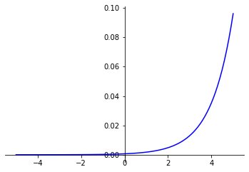
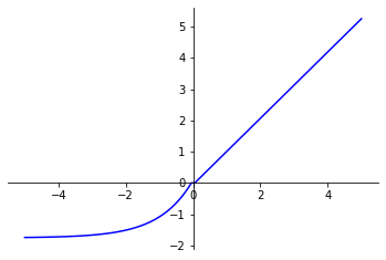
Softplus function is a “soft” approximation of the ReLU function.

With positive input values, the Softplus function behaves, with a few exceptions, in the same way as ReLU. However, for negative input values, the Softplus function doesn’t apply a filter like ReLU, but tends towards zero.

Softplus_function(x) = log(exp(x) + 1)

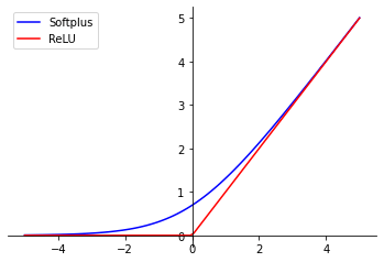
This asymptotic curve enables more stable gradients to be obtained during backpropagation, which can improve model training.

How to use the Softplus function with Keras :

tf.keras.activations.softplus(x)

Softsign

Softsign function is used to apply normalization to input values.

It produces output values between -1 and 1.

Softsign_function(x) = x / (abs(x) + 1)

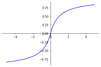
The Softsign function also preserves the sign (positive or negative) of input values. A property that can be useful for certain tasks, but which is not often used.

How to use the Softsign function with Keras :

tf.keras.activations.softsign(x) 

tanh

tanh function can be used to apply normalization to input values. It can also be used instead of the Sigmoid function in the last layer of a binary classification model.

It gives a result between -1 and 1.

tanh_function(x) = ((exp(x) – exp(-x))/(exp(x) + exp(-x)))

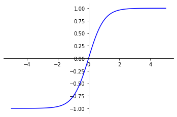
In binary classification, the result obtained after using the tanh function cannot be directly interpreted as a probability, as it will lie between -1 and 1. It can then be modified to be observed in the same way as a probability.

How to use the tanh function with Keras :

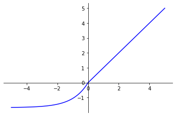
tf.keras.activations.tanh(x)

ELU

Exponential Linear Unit (ELU) function is a variation of the ReLU function.

ELU behaves in the same way as ReLU for positive input values. However, for negative input values, ELU gives smooth values below 0.

ELU_function(x) =

• if x > 0: x
• if x < 0: alpha * (exp(x) - 1)

with :

• alpha > 0

The ELU activation function has shown promising results in various Deep Learning applications. This smoothed alternative to the ReLU function overcomes some of its limitations while retaining its beneficial properties for training neural networks.

How to use the ELU function with Keras :

tf.keras.activations.elu(x, alpha=1.0)

• alpha: a variable used to control the slope of ELU when x < 0. The greater the alpha, the steeper the curve. This value must be greater than 0

SELU

Scaled Exponential Linear Unit (SELU) function is an improvement on ELU.

SELU multiplies a scale variable with the result of function ELU. This operation is designed to promote normalization of output values.

SELU_function(x) =

• if x > 0: return scale * x
• if x < 0: return scale * alpha * (exp(x) - 1)

with, as constant :

• alpha = 1.67326324
• scale = 1.05070098

Like ELU, SELU overcomes some of ReLU’s limitations while retaining its beneficial properties for training neural networks.

How to use ELU with Keras :

tf.keras.activations.selu(x)

Note: When using SELU, layer weights must be initialized with 'lecun_normal'.

model.add(tf.keras.layers.Dense(64, kernel_initializer='lecun_normal', activation='selu'))

Customized ActivationFunctions

When researching or experimenting, you may find that the predefined activation functions in the Python libraries don’t meet your needs.

For example, if the activation functions you select don’t produce the expected result, or if you wish to apply specific non-linear transformations.

In this case, you can create your own activation functions. There are two rules to bear in mind:

• An activation function must be non-linear
• An activation function takes a tensor as input.

Note: Classic Python libraries provide functions that can be applied to real numbers. For example, in math.exp(x), x is a real number. But to create an activation function, you’ll need to use functions applicable to tensors. For example, in tensorflow.math.exp(x), x is a tensor.

How to create an activation function with Keras :

from keras import backend as K

def maFonction(x, beta=1.0):
    return x * K.sigmoid(beta * x)

How to use a custom activation function with Keras :

from keras.layers.core import Activation

model.add(layers.Dense(16))
model.add(Activation(maFonction))

Note: an activation function can be added to a model, independently of the use of a layer, as in the code above. It will then apply to the output of each neuron in the previous layer.

Caution: If you save a model using a customized activation function, to reuse it in another program, you’ll need to redefine the same activation function!

Conclusion

Activation functions play a crucial role in neural networks. By applying a non-linear transformation to the data passing through the model, they enable the spatial representation of the data to be modified.

It is this particularity of activation functions that gives Deep Learning algorithms their power. In many cases, neural networks outperform traditional Machine Learning algorithms.

Several activation functions exist. It’s important to know how to differentiate between them, as they don’t apply the same transformations to the data. As a result, if you use an activation function that isn’t suited to the task you’re facing, it can reduce your model’s performance to ashes.

So that you don’t fall into the trap, I’ve prepared a table clarifying which activation functions to choose according to the type of task you’re facing, as well as a summary of this article. To access it, click here :

GET MY ACTION PLAN