Sentences Embedding Visualization – How to do it the Best Way

In this article, we propose a tutorial to efficiently create Sentences Embedding Visualization; also called TSNE applied to NLP.

For this, we use the GoEmotions dataset from Google which contains more than 58,000 sentences labeled according to 27 emotions. For each sentence only ONE emotion is associated, so it’s a multi-class classification problem…

… but you can easily adapt this tutorial to any type of classification !

One more point before we start,

Embedding is the computer representation of a sentence. It is used to make the machine understand the language of Man.

To visualize the Embedding of sentences, it is necessary first to create this Embedding.

Therefore, this tutorial will have 3 parts :

Preparing the data – GoEmotions

Prerequisite : We recommend that you use a computer with a GPU or that you code on Google Colab and activate the integrated GPU for free.

To start this tutorial, we load the whole GoEmotions dataset thanks to the Google API. This dataset is decomposed in 3 csv files :

!wget -P data/full_dataset/ https://storage.googleapis.com/gresearch/goemotions/data/full_dataset/goemotions_1.csv &> /dev/null
!wget -P data/full_dataset/ https://storage.googleapis.com/gresearch/goemotions/data/full_dataset/goemotions_2.csv &> /dev/null
!wget -P data/full_dataset/ https://storage.googleapis.com/gresearch/goemotions/data/full_dataset/goemotions_3.csv &> /dev/null

Then, we create a Pandas dataframe which will contain these 3 csv files. We remove the columns that we’rre not going to use and we delete sentences that appear more than once in the dataset :

import numpy as np
import pandas as pd

df1 = pd.read_csv('/content/data/full_dataset/goemotions_1.csv')
df2 = pd.read_csv('/content/data/full_dataset/goemotions_2.csv')
df3 = pd.read_csv('/content/data/full_dataset/goemotions_3.csv')
df = pd.concat([df1, df2, df3], sort=False)
df.drop(['id', 'link_id','parent_id','created_utc','rater_id','example_very_unclear'], axis=1, inplace=True)
df.drop_duplicates(subset=['text', 'author', 'subreddit'], inplace=True)
df.reset_index(inplace=True, drop=True)

After this short processing, we can examine our dataset:

len(df)

Output : 58009

Data

We have a dataset of 58 009 sentences, we may display the first lines to see more details of these data :

df.head(1)

We can see that the dataframe is quite illegible. In addition to that, there are still some columns that are not going to be useful to us like the one containing the name of the author.

By the way, this dataset is taken from the online forum Reddit, you can find all kinds of sentences… quite wacky… you are warned !

We’ll create a second dataframe, which will be the one we will really use during this tutorial :

df_analysis = df[['text']]

⬆ We add the sentences to this new dataframe.

Then, we also want to have the emotions associated with each of these sentences.

The problem is that they are encoded as numbers : 1 if the emotion is present, 0 if it is not.

I suggest you to simplify all this with this line of code :

df_analysis['text_emotion'] = df.drop(columns=['text','author','subreddit'], axis=1, inplace=False).idxmax(axis=1)

Let’s display the resulting dataframe :

df_analysis.head(1)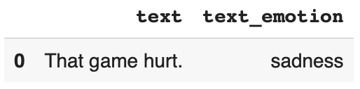

It is much more clearer ! We have here a dataframe containing 2 columns : one for the sentences, one for the associated emotion.

Yet one last step since…

… by creating an Embedding, we actually make Deep Learning. This DL model will learn on our data and depending on the power of your GPU, it can take time.

To speed up the learning process, I suggest to reduce the amount of data. We will focus only on 7 emotions associated with 1000 sentences each :

df_analysis = pd.concat([df_analysis[df_analysis['text_emotion'] == 'joy'].iloc[:1000],
                         df_analysis[df_analysis['text_emotion'] == 'sadness'].iloc[:1000],
                         df_analysis[df_analysis['text_emotion'] == 'curiosity'].iloc[:1000],
                         df_analysis[df_analysis['text_emotion'] == 'neutral'].iloc[:1000],
                         df_analysis[df_analysis['text_emotion'] == 'love'].iloc[:1000],
                         df_analysis[df_analysis['text_emotion'] == 'amusement'].iloc[:1000],
                         df_analysis[df_analysis['text_emotion'] == 'embarrassment'].iloc[:1000]
                         ])

The 27 emotions recorded are: admiration, amusement, anger, annoyance, approval, benevolence, confusion, curiosity, desire, disappointment, disapproval, disgust, embarrassment, excitement, fear, gratitude, sorrow, joy, love, nervousness, optimism, pride, achievement, relief, remorse, sadness, surprise, neutral.

Feel free to choose among those that appeal to you… the final results are particularly interesting!

Transfer Learning – BERT

Importing Bert

As I told you above, in this tutorial we use Deep Learning. And as the dataset is particularly complex, we will use the famous BERT model.

In fact, we will do Transfer Learning. That is to say we will use a version of BERT that has already been trained.

Thus we will acquire the performances it has already obtained, then adapt it (train it again) on our data!

This is what we call Transfer Learning.

We have already discussed Transfer Learning with BERT in this article, so we’ll skip that topic and move on to the heart of this tutorial!

We load BERT :

import tensorflow_hub as hub

module_url = "https://tfhub.dev/tensorflow/bert_en_uncased_L-12_H-768_A-12/1"

bert_layer = hub.KerasLayer(module_url, trainable=True)

Next, we install the dependencies:

!pip install bert-tensorflow &> /dev/null
!pip install sentencepiece &> /dev/null

And the code to process our data :

import tokenization
import numpy as np
import tensorflow as tf
from tensorflow.keras import layers
from tensorflow.keras.optimizers import Adam
from tensorflow.keras.models import Model
from tensorflow.keras.callbacks import ModelCheckpoint
# The 4 next lines allows to prevent an error due to Bert version
import sys
from absl import flags
sys.argv=['preserve_unused_tokens=False']
flags.FLAGS(sys.argv)

def bert_encode(texts, tokenizer, max_len=512):
    all_tokens = []
    all_masks = []
    all_segments = []
    
    for text in texts:
        text = tokenizer.tokenize(text)
            
        text = text[:max_len-2]
        input_sequence = ["[CLS]"] + text + ["[SEP]"]
        pad_len = max_len - len(input_sequence)
        
        tokens = tokenizer.convert_tokens_to_ids(input_sequence)
        tokens += [0] * pad_len
        pad_masks = [1] * len(input_sequence) + [0] * pad_len
        segment_ids = [0] * max_len
        
        all_tokens.append(tokens)
        all_masks.append(pad_masks)
        all_segments.append(segment_ids)
    
    return np.array(all_tokens), np.array(all_masks), np.array(all_segments)

vocab_file = bert_layer.resolved_object.vocab_file.asset_path.numpy()
do_lower_case = bert_layer.resolved_object.do_lower_case.numpy()
tokenizer = tokenization.FullTokenizer(vocab_file, do_lower_case)

train_input = bert_encode(df_analysis.text.values, tokenizer, max_len=100)
train_labels = df_analysis.text_emotion.values

Multiclass Classification with Bert

Again, all the code you see here is detailed in this article, feel free to consult it if you want to understand how to use BERT.

However, I draw your attention to the part below which is different from our BERT tutorial, especially the 3 lines with :

• “flatten”
• “output_flatten”
• “out”

def build_model(bert_layer, max_len=512):
    input_word_ids = layers.Input(shape=(max_len,), dtype=tf.int32, name="input_word_ids")
    input_mask = layers.Input(shape=(max_len,), dtype=tf.int32, name="input_mask")
    segment_ids = layers.Input(shape=(max_len,), dtype=tf.int32, name="segment_ids")

    _, sequence_output = bert_layer([input_word_ids, input_mask, segment_ids])
    clf_output = sequence_output[:, 0, :]

    flatten = layers.Flatten(name='flatten')
    output_flatten = flatten(clf_output)

    out = layers.Dense(len(np.unique(train_labels)), activation='sigmoid')(output_flatten)
    
    model = Model(inputs=[input_word_ids, input_mask, segment_ids], outputs=out)
    model.compile(Adam(lr=2e-6), loss='binary_crossentropy', metrics=['accuracy'])
    
    return model

model = build_model(bert_layer, max_len=100)

At the “flatten” line, we define the Embedding layer. This is what will translate the sentence into computer language.

Our objective is to train the model so that it optimizes the Embedding layer and so that we can get a good representation of the data.

If we did not train the model, it would still do this Embedding but without linking the sentences to the emotions.

When training, the model modifies each of its layers. Once the layers are modified and optimized, it can understand from a sentence, the emotion that is linked to it.

So by learning, it optimizes its Embedding. By the way, you can try it on your side and see that if the model is badly trained, the Embedding Visualization will give nothing meaningful.

Parenthesis closed ! The result will be at the end of this article 🔥

At the line “output_flatten”, we use the previously created embedding layer.

And finally, the “out” layer, where instead of having Dense(2, …) we have Dense(len(np.unique(train_labels)) …).

In fact this number indicates the number of outputs of the model. We used 2 for a Binary Classification.

Here we have a Multiclass Classification. If you choose to analyze the whole dataset (the 27 emotions) you can directly indicate 27.

Training BERT

But since this number depends on the power of our GPU, we decided to opt for an adaptive solution with len(np.unique(train_labels)).

This solution measures the number of emotions contained in your dataset. We have 7 emotions so this code automatically indicates “7“. So, no need to change this piece of code if we add or remove emotions to our dataframe!

Speaking of emotions… we also need to translate them into computer language.

Since they are categorical data, this is much easier thanks to the get_dummies() function :

label_dummy = pd.get_dummies(train_labels)

Feel free to display the result to understand the transformations we apply at each moment :

label_dummy.head(2)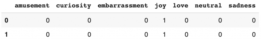

Finally, we can train our model and this is where our GPU will show its worth :

train_history = model.fit(
    train_input, label_dummy,
    validation_split=0.2,
    epochs=10,
    batch_size=32
)

Almost 30 minutes of learning on my side ! I recommend you to check the final accuracy of your model.

The higher it is, the more efficient the Embedding Visualization will be !

Anyway, we can FINALLY move on to…

TSNE – Visualization of Embedding of sentences

Extract the Embedding

As I said before, we want to extract the result from the Embedding layer.

To do this, we recreate a model from the old one by including all its layers up to “flatten”, the Embedding layer:

intermediate_layer_model = Model(inputs=model.input,
                                 outputs=model.get_layer('flatten').output)

Then we send our data into the newly created model to have the result !

sentence_embedded = intermediate_layer_model.predict(train_input)

That’s it ! We have our sentence embedding.

Now we retrieve the emotions associated with each of these sentences:

labels_emotion = df_analysis.text_emotion

Here we can check the dimensions of the embedding…

sentence_embedded.shape

… and that of the emotions :

labels_emotion.shape

On my side I have (6433, 768) and (6433,).

So 6433 sentences for 6433 emotions, it’s a match !

TSNE

(Shouldn’t we have 7000 sentences? – In fact, in our dataset, each emotion is associated with a different number of sentences. We can therefore imagine that some are linked to less than 1000 sentences. This does not raise any issue for our algorithm, let’s keep going !)

To visualize the Embedding, we must project the sentences on a 2 (or 3) dimensional axis.

Here we have a dimension of (, 768). It is much too much! And this is where the TSNE comes in.

The TSNE is an algorithm allowing to reduce the dimension of an array (matrix) while preserving the important information contained inside.

It can be used via the sklearn library… and for the curious, yes it is a Machine Learning algorithm. It uses in fact the KNN.

But enough of theory ! It is the practice that drives us in this tutorial:

import numpy as np
from sklearn.manifold import TSNE

X = list(sentence_embedded)

X_embedded = TSNE(n_components=2).fit_transform(X)

We have thus reduced the dimension of our Embedding.

Now, to organize all this, we create a dataframe containing the 2D Embedding of the sentences and their emotions :

df_embeddings = pd.DataFrame(X_embedded)
df_embeddings = df_embeddings.rename(columns={0:'x',1:'y'})
df_embeddings = df_embeddings.assign(label=df_analysis.text_emotion.values)

We will also add the unmodified base sentences, to make the visualization easier :

df_embeddings = df_embeddings.assign(text=df_analysis.text.values)

If you have reached this step, congratulations ! It’s a long tutorial, but it allows to have a particularly interesting result.

Let’s display it without further delay !

Display Embedding

For that, we use Plotly. We indicate the dataframe to be displayed, the columns to be taken as axes, the columns to be taken as label and finally the hover_data allows to associate each of the projected points to their respective sentences :

import plotly.express as px

fig = px.scatter(
    df_embeddings, x='x', y='y',
    color='label', labels={'color': 'label'}
    hover_data=['text'], title = 'GoEmotions Embedding Visualization')
fig.show()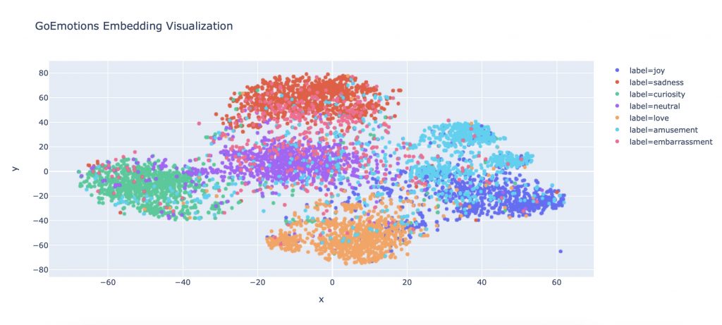

And that’s it ! You have successfully done your first sentence embedding !

You can now visualize how the Deep Learning algorithm represents the relationships between sentences and emotions.

Moreover, you can see that it doesn’t simply make separations between each emotion.

On the contrary, the more the sentences have a similar emotion, the closer they are and vice versa.

Thus, we have the emotions ‘love’ and ‘sadness’ which are clearly separated but we can also see ‘love’, ‘joy’, and ‘amusement’ almost merging in some places.

Deep Learning not only interprets the emotions according to the sentences but we can see that it really understands the similarity of the words and their emotional values.

Going further

To go further, we can obviously choose more emotions, more sentences (for that, get a good GPU!) but we can also refine the Embedding display by adding dimensions to this visualization.

Let’s add for example the size of each sentence in our dataframe:

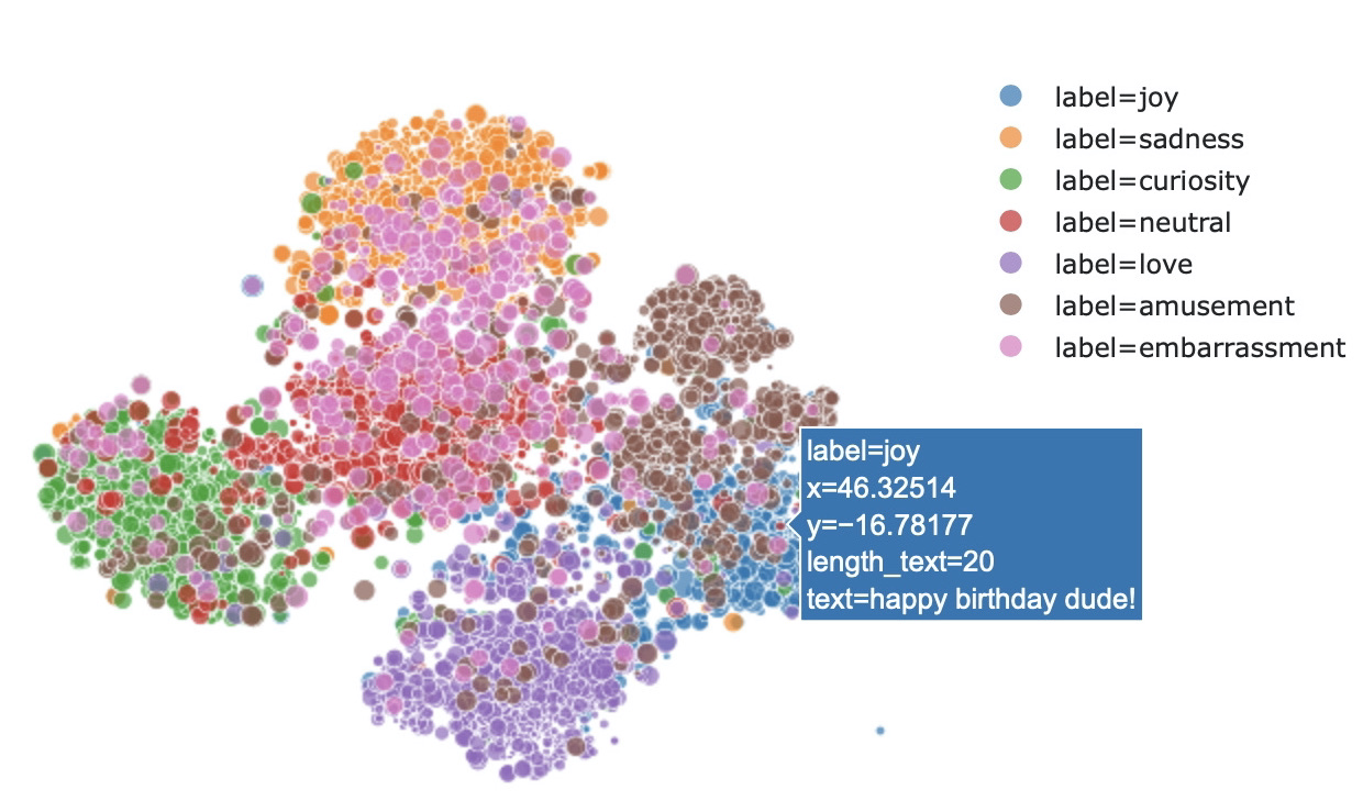
df_embeddings['length_text'] = df_embeddings[['text']].applymap(lambda x : len(x))

We can integrate this dimension in our display. So the longer the sentence will be, the bigger the point that represents it will be :

import plotly.express as px

fig = px.scatter(
    df_embeddings, x='x', y='y',
    color='label', labels={'color': 'label'},
    size = 'length_text', size_max = 10, template = 'simple_white',
    hover_data=['text'], title = 'GoEmotions Embedding Visualization')
fig.show()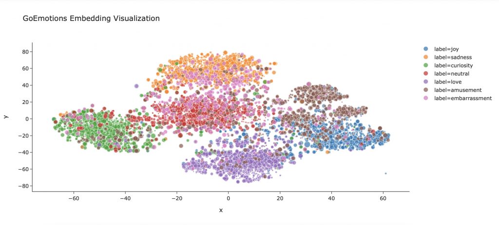

Feel free to add several dimensions to this visualization.

Or simply change the design. This is not a technical approach but it can change the perception of the graphic. Here we use the template ‘simple_white’, not bad isn’t it ?

This is the end of this article. We hope you enjoyed it !

See you soon in a next tutorial 😉

sources :

• Google’s GoEmotions dataset