Easy Tutorial – Object detection on image in PyTorch part 2

How to code a Deep Learning algorithm for object detection with the PyTorch library ? That’s what we’ll see in this article !

This article is part of a series on Binary Classification models with PyTorch with :

• first part on normalization (available here)
• second part on Deep Learning model

We will use the data from the first part, feel free to consult it before continuing the reading

Let’s continue this series by looking at creation and training of a Deep Learning model with PyTorch.

Build a PyTorch Model

Net() class

As you know Python is an object oriented programming language, that is to say that in Python we can(must…?) create our own objects and functions.

In this sense, we say that PyTorch is ‘Pythonic’: it uses the same principles as Python’s object-oriented.

With Keras we can call functions quite easily, with PyTorch we will have to create objects in most cases… and that’s good news !

For those who are not used to object-oriented programming, this may seem confusing, but the sooner we get into it, the sooner we will be able to create our own objects, our own libraries and adapt to all situations !

If you want to learn more about object-oriented programming in Python I recommend this site.

For the others, let’s continue ! 🙂

We are going to build a class that will allow to initialize a neural network as an object.

For this we define a constructor (init): when calling the object, we will get a variable that contains each of the attributes specified in this constructor. This is where we define the fully connected layers of our neural network.

Then we define a function that will activate our model : the forward function. It allows to connect the different layers between them and to transmit the data along the neural network.

import torch.nn as nn
import torch.nn.functional as F

class Net(nn.Module):
  def __init__(self):
    super().__init__()
    self.conv1 = nn.Conv2d(3, 16, kernel_size=3, padding=1)
    self.conv2 = nn.Conv2d(16, 8, kernel_size=3, padding=1)
    self.fc1 = nn.Linear(8 * 8 * 8, 32)
    self.fc2 = nn.Linear(32, 2)

  def forward(self, x):
    out = F.max_pool2d(torch.tanh(self.conv1(x)), 2)
    out = F.max_pool2d(torch.tanh(self.conv2(out)), 2)
    out = out.view(-1, 8 * 8 * 8)
    out = torch.tanh(self.fc1(out))
    out = self.fc2(out)
    return out

Clarification

Our object is a child of the module nn.Module. This is specified when we write Net(nn.Module) and when we call the function super().

In other words super() connects our Net() object to the nn.Module class (which becomes its parent).

Then we call all the layers fully connected in our constructor : the convolution layers and the linear layers.

Then we connect these layers with the Max Pooling layer, out.view (the equivalent of Flatten in Keras), and the activation functions (here tanh).

Even if our model is not yet trained we may use it to see if everything is going well.

For this we define a random tensor that we pass in our model :

import torch
random_tensor = torch.rand((1, 3, 32, 32))

nn_test = Net()
result = nn_test(random_tensor)
print(result)

On a bien en sortie deux float qui, une fois que le modèle sera entraîné, correspondront chacun à la probabilité d’être dans la classe ‘cerf’ et dans la classe ‘cheval’.

We have two floats in output which, once the model is trained, will each correspond to the probability of being in the class ‘deer’ and in the class ‘horse’.

Training a PyTorch Model

Using CPU

Training loop

In PyTorch there is no equivalent to Keras.fit(), you have to create your own training loop.

This training loop is explained in the code below.

import datetime

def training_loop(n_epochs, optimizer, model, loss_fn, train_loader):
  for epoch in range(1, n_epochs + 1):
      loss_train = 0.0

      for imgs, labels in train_loader:
        outputs = model(imgs)
        loss = loss_fn(outputs, labels)
        optimizer.zero_grad()
        loss.backward()
        optimizer.step()
        loss_train += loss.item()

      if epoch == 1 or epoch % 10 == 0:
        print('{} Epoch {}, Training loss {}'.format(
            datetime.datetime.now(), epoch,
            loss_train / len(train_loader)))

In fact the process is quite simple. At each epoch you have to initialize the loss (loss_train) to 0. Then :

• Use the model on our data (make a prediction)
• Calculate the loss (the error between our prediction and the reality)
• Set the gradient to zero
• Compute the backpropagation (compute the gradient)
• Update the parameters (via the gradient)
• Update the global loss (loss_train)

Then we can display the result at each epoch. Here we do it every 10 epochs.

For this we divide the global loss by the length of our dataset.

Training

We initialize our three main objects :

• the model
• an optimization function (here we take the classical Stochastic Gradient Descent)
• the loss function

import torch.optim as optim

model = Net()
optimizer = optim.SGD(model.parameters(), lr=1e-2)
loss_fn = nn.CrossEntropyLoss()

Then for the data, we will use a very special object called DataLoader.

When training a model, we usually want to batch our data, mix the data at each epoch to reduce overfitting, and use Python’s multiprocessing to speed up the calculations.

DataLoader is an iterable object that eases this task for us in a simple module (also called API).

import torch

train_loader = torch.utils.data.DataLoader(cifar2, batch_size=64,
                                            shuffle=True)
val_loader = torch.utils.data.DataLoader(cifar2_val, batch_size=64,
                                         shuffle=False)

We can finally train our model by indicating the desired parameters in our training loop!

training_loop(
    n_epochs = 100,
    optimizer = optimizer,
    model = model,
    loss_fn = loss_fn,
    train_loader = train_loader)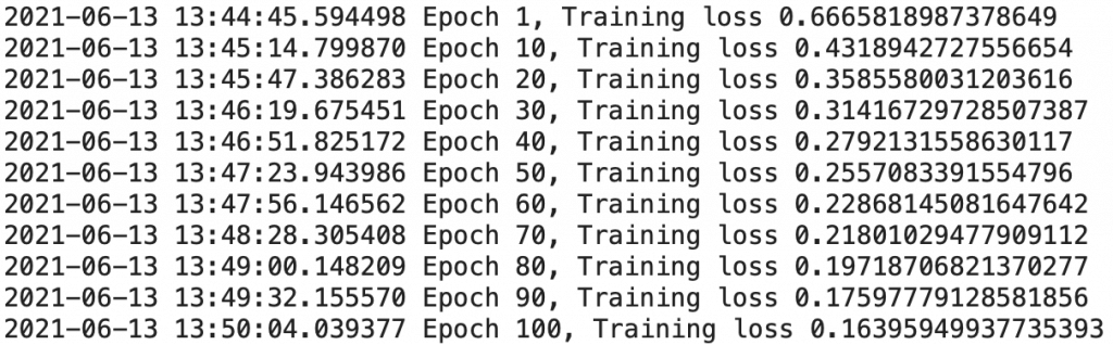

Our training is finished. We get a loss of 0.151, not bad for a first training!

What if we pushed the performance analysis a little further?

Validation

In the following function, we calculate the accuracy of the model on our training data and on our validation data, to check that there is no overfitting.

Overfitting is the fact that a model becomes so specialized on its training data that it becomes inefficient on other data, real data.

def validate(model, train_loader, val_loader):
    for name, loader in [("train", train_loader), ("val", val_loader)]:
      correct = 0
      total = 0
      with torch.no_grad():
          for imgs, labels in loader:
            outputs = model(imgs)
            _, predicted = torch.max(outputs, dim=1)
            total += labels.shape[0]
            correct += int((predicted == labels).sum())

      print("Accuracy {}: {:.2f}".format(name , correct / total))

For each batch of our DataLoader (train & val), the function looks at the number of right predictions.

validate(model, train_loader, val_loader)

We obtain 0.92 for the train and 0.88 for the val.

In addition to being very close (which indicates that there is no overfitting), these accuracies are also really high, our Deep Learning model is particularly efficient for this classification !

Saving / Loading the weights

We can now save the weights of our model to use elsewhere without having to train it again ! 🙂

torch.save(model.state_dict(), 'birds_vs_airplanes.pt')

And here is the code to use it in another program.

Note that we will also have to transfer our neural network, the Net() object.

loaded_model = Net()
loaded_model.load_state_dict(torch.load('birds_vs_airplanes.pt'))

There we go ! We can now use our Deep Learning model anywhere !

Using GPU

Initialize the GPU

With PyTorch, we can accelerate the training time of our Deep Learning model if we have a GPU.

The Graphics Processing Unit or graphic processor allows to make several calculations at the same time, in parallel. Simply put, a GPU allows to greatly accelerate the computation time, ideal for Deep Learning!

We remind you that you can access a GPU for free using Google Colab 😉

After modifying the Execution settings in Colab, you need to use this code brick to use the cuda GPU with PyTorch:

device = (torch.device('cuda') if torch.cuda.is_available()
                  else torch.device('cpu'))

print(f"Training on device {device}.")

Training

Once we have initialized the GPU, all we have to do is to tell PyTorch that we want the computations to be performed on it in our training loop.

To do this we use the to() function.

When we code: imgs.to(torch.device(‘cuda’)); we tell PyTorch to perform the calculations of the imgs tensor on the ‘cuda’ GPU.

By default, PyTorch tensors are computed on CPU.

import datetime

def training_loop(n_epochs, optimizer, model, loss_fn, train_loader):
  for epoch in range(1, n_epochs + 1):
    loss_train = 0.0

    for imgs, labels in train_loader:
      imgs = imgs.to(device=device)
      labels = labels.to(device=device)

      outputs = model(imgs)
      loss = loss_fn(outputs, labels)
      optimizer.zero_grad()
      loss.backward()
      optimizer.step()
      loss_train += loss.item()
    
    if epoch == 1 or epoch % 10 == 0:
      print('{} Epoch {}, Training loss {}'.format(
          datetime.datetime.now(), epoch,
          loss_train / len(train_loader)))

We notice that the code is exactly like our CPU version, except for the two lines that transfer the ‘imgs’ and ‘labels’ inputs to the GPU.

When calling the Net() object, you must also specify the transfer to the GPU :

import torch.optim as optim

model = Net().to(device=device)
optimizer = optim.SGD(model.parameters(), lr=1e-2)
loss_fn = nn.CrossEntropyLoss()

Data from the DataLoader will be transferred to the GPU in each epoch, so we leave the initialization unchanged :

import torch

train_loader = torch.utils.data.DataLoader(cifar2, batch_size=64,
                                            shuffle=True)
val_loader = torch.utils.data.DataLoader(cifar2_val, batch_size=64,
                                         shuffle=False)

We launch the training which, we can see it, is much faster than on CPU !

training_loop(
    n_epochs = 100,
    optimizer = optimizer,
    model = model,
    loss_fn = loss_fn,
    train_loader = train_loader)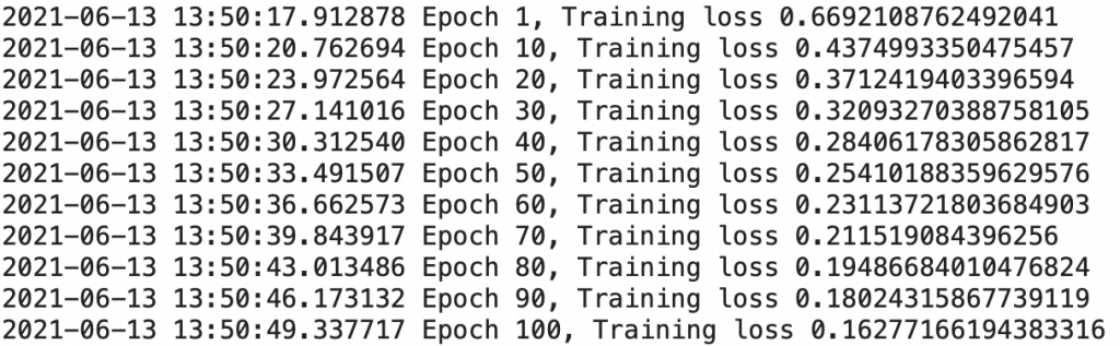

Furthermore, we must transfer to the GPU the imgs and label variables of our validation function :

def validate(model, train_loader, val_loader):
    for name, loader in [("train", train_loader), ("val", val_loader)]:
      correct = 0
      total = 0
      with torch.no_grad():
          for imgs, labels in loader:
            outputs = model(imgs.to(device))
            _, predicted = torch.max(outputs, dim=1)
            total += labels.shape[0]
            correct += int((predicted == labels.to(device)).sum())

      print("Accuracy {}: {:.2f}".format(name , correct / total))

And now, validate our model:

validate(model, train_loader, val_loader)

Testing the model

Now that the training is completed, wee may test our model on an image, let’s take this one :

import matplotlib.pyplot as plt

img, _ = cifar2[290]

plt.imshow(unorm(img).permute(1, 2, 0))
plt.show()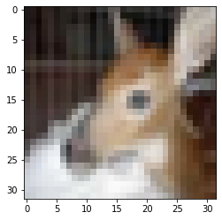

Afterwards, to predict the label of this image we use our model through this piece of code :

# evaluate model:
loaded_model.eval()

with torch.no_grad():
    out_data = loaded_model(img.unsqueeze(0).to(device=device))

print(out_data)
print(class_names)

The larger the result, the higher the probability of belonging to the class and vice versa.

Here our model predicts with a high probability that the image belongs to the class ‘deer’ !

Saving / Loading the weights

To save the weights of our model, the process is the same as with CPU :

torch.save(model.state_dict(), 'birds_vs_airplanes_wgpu.pt')

However, to load them it will be necessary to indicate the GPU transfer when calling Net() and the parameter map_location=device when loading the weights :

loaded_model = Net().to(device=device)
loaded_model.load_state_dict(torch.load('birds_vs_airplanes_wgpu.pt',
                                        map_location=device))

sources :

• L. Antiga, Deep Learning with PyTorch (2020, Manning Publications) :
  • our affiliate link – Germany
  • our affiliate link – United Kingdom
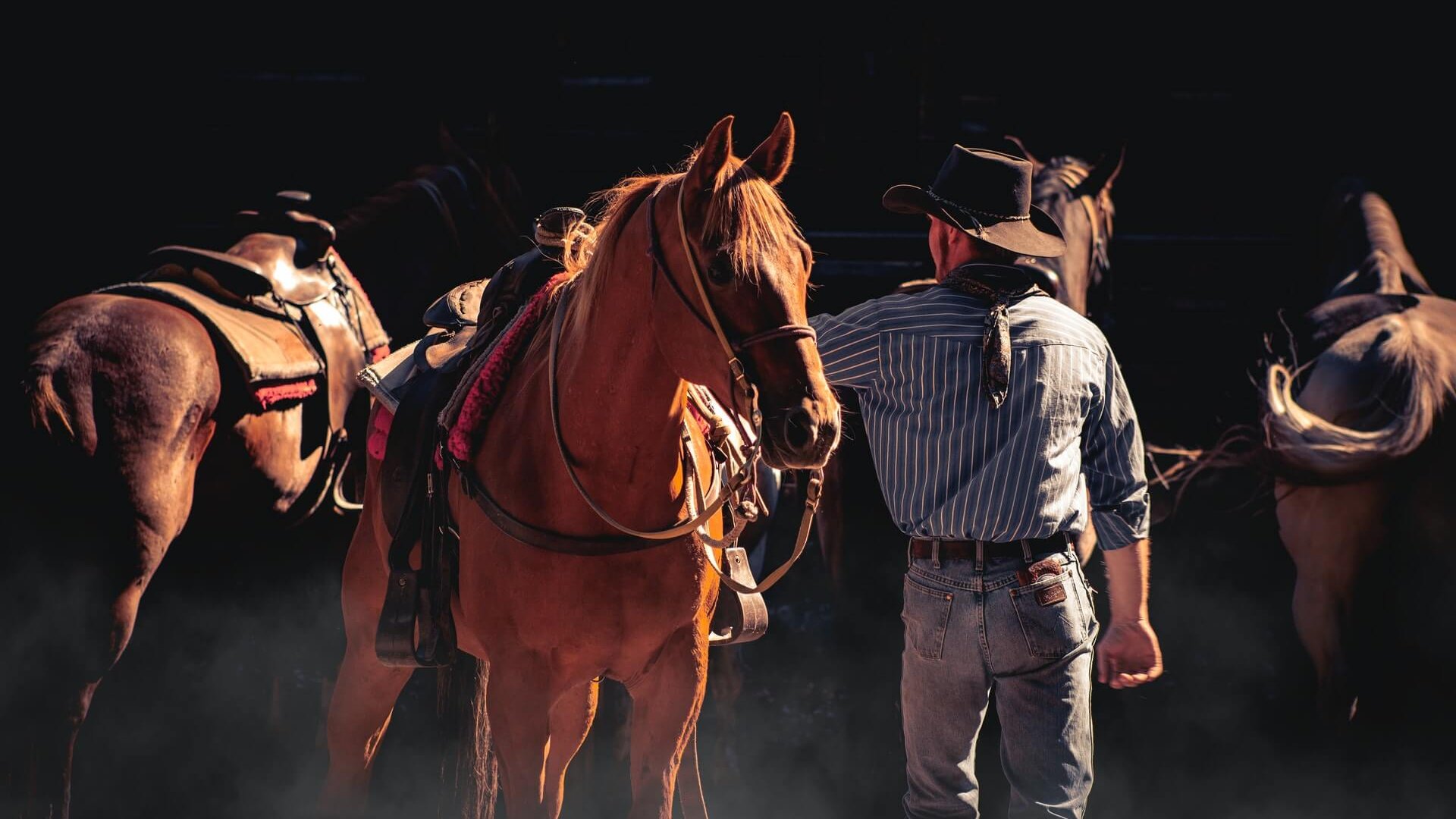
• Photo by Diana Parkhouse on Unsplash