Why and How to normalize data – Object detection on image in PyTorch Part 1

Today we will see how normalize data with PyTorch library and why is normalization crucial when doing Deep Learning.

In fact this article is part of a series on Binary Classification models in PyTorch with :

• a first part on normalization
• a second part on Deep Learning models (available here)

Without further introduction, let’s begin this first part on data normalization.

Loading data

First of all we will load the data we need.

We use for that the datasets module.

It’s a module integrated to PyTorch that allows to quickly load datasets. Ideal to practice coding !

The dataset that interests us is called CIFAR-10. It is composed of 60 000 images in RGB color and size 32×32; they are divided into 10 classes (plane, automobile, bird, cat, deer, dog, frog, horse, boat, truck), with 6 000 images per class.

from torchvision import datasets
from torchvision import transforms

data_path = '../data-unversioned/p1ch7/'

cifar10 = datasets.CIFAR10(
    data_path, train=True, download=True,
    transform=transforms.ToTensor()
    )

Several parameters are specified:

• data_path, the directory where the cifar-10 dataset will be saved
• train = True, create the dataset from the training set, if False create from the test set.
• download = True, downloads the dataset from the internet and places it in the root directory. If the dataset is already downloaded, it is not downloaded again.
• transform = transforms.ToTensor(), allows to initialize the images directly as a PyTorch Tensor (if nothing is specified the images are in PIL.Image format)

Verifying the data

Let’s be a bit more precise, we have a variable cifar10 which is a dataset containing tuples.

These tuples are composed of :

• a tensor (which represents the image)
• an int which represents the label of the image

img_t, index_label = cifar10[5]
type(img_t), type(index_label)

We have recovered one of the images of the dataset, let’s display it !

We recall that an image tensor is in the format Color X Height X Width. To display the image, it is necessary to change its format to Height X Width X Color.

To do so, we use the permute() function.

import matplotlib.pyplot as plt

plt.imshow(img_t.permute(1, 2, 0))
plt.show()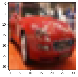

We also may display the label associated with the image:

index_label

The index_label variable is equal to 1. In fact we have retrieved the index that will allow us to know the name of the label.

For that, we just have to refer to this list :

label_names = ['airplane', 'automobile', 'bird', 'cat', 'deer', 'dog', 'frog', 'horse', 'ship', 'truck']
label_names[index_label]

Our image has the label ‘automobile’. So far, everything seems to be consistent !

Normalizing data

Normalizing data is a step often forgotten by Data Scientists, even though it is essential to build a good Machine Learning algorithm.

Normalization is the fact of modifying the data of each channel/tensor so that the mean is zero and the standard deviation is one.

We show you an example with the normalization of a list below :

We show you an example below with the normalization of a list below…

…first, we calculate the mean and the standard deviation :

import numpy as np

l = [60, 9, 37, 14, 23, 4]

np.mean(l), np.std(l)

We obtain : (24.5, 19.102792117035317)

In fact, this calculation will allow us to apply the following normalization formula on each element of the list:

(element – mean) / standard deviation

l_norm = [(element - np.mean(l)) / np.std(l) for element in l]

print(l_norm)

We obtain : [1.86, -0.81, 0.65, -0.55, -0.08, -1.07]

Our list is now normalized.

We can check that the mean is 0 and the standard deviation is 1:

np.mean(l_norm), np.std(l_norm)

We obtain : (0.0, 1.0)

But why do we want to normalize our data?

In fact there are two main reasons :

• normalizing data includes them in the same range as our activation functions, usually between 0 and 1. This allows for less frequent non-zero gradients during training, and therefore the neurons in our network will learn faster.
• by normalizing each channel so that they have the same distribution, we ensure that the channel information can be mixed and updated during the gradient descent (back propagation) using the same learning rate.

Reminder : we call a channel a group of tensor. In our case each image corresponds to a tensor.

The PyTorch advantage

Normalize Data Manually

With PyTorch we can normalize our data set quite quickly.

We are going to create the tensor channel we talked about in the previous part.

To do this, we use the stack() function by indicating each of the tensors in our cifar10 variable :

import torch

imgs = torch.stack([img_t for img_t, _ in cifar10], dim=3)
imgs.shape

We obtain a channel that contains 50 000 images in 3x32x32 format.

In fact this channel is a tensor. It is a tensor which contains other tensors 😉

Thanks to this channel, we can calculate the average of all the tensors :

imgs.view(3, -1).mean(dim=1)

We obtain three mean : tensor([0.4914, 0.4822, 0.4465])

Each one represents the mean of each color : R G B.

Same thing for the standard deviation :

imgs.view(3, -1).std(dim=1)

We obtain three standard deviations : tensor([0.2470, 0.2435, 0.2616])

No need to rewrite the normalization formula, the PyTorch library takes care of everything!

We simply use the Normalize() function of the transforms module by indicating the mean and the standard deviation :

norm = transforms.Normalize((0.4915, 0.4823, 0.4468), (0.2470, 0.2435, 0.2616))

We can then normalize an image…

out = norm(img_t)

… or all images of the channel at the same time:

imgs_norm = torch.stack([norm(img_t) for img_t, _ in cifar10], dim=3)

Finally we can verify that our channel is well normalized with a mean of 0 and a standard deviation of 1 :

print(imgs_norm.mean(), imgs_norm.std())

Normalize Data Automatically

If we know the mean and the standard deviation we can directly apply the normalization when loading the tensors.

You just have to add the Normalize() function when we initialize the dataset as follows:

transformed_cifar10 = datasets.CIFAR10(
    data_path, train=True, download=True,
    transform=transforms.Compose([
        transforms.ToTensor(),
        transforms.Normalize((0.4915, 0.4823, 0.4468),
                             (0.2470, 0.2435, 0.2616))
        ]))

As you can see, if you want to call the transforms module several times on an object you have to group these calls in the Compose() function

The Compose() function allows you to perform several transformations at the same time.

Denormalizing Data

So we have our normalized dataset ready to be used… but before that let’s display our normalized image to see what it looks like:

import matplotlib.pyplot as plt

img, ind = transformed_cifar10[12]

plt.imshow(img.permute(1, 2, 0))
plt.show()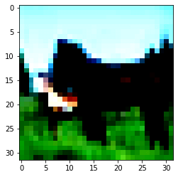

The image is quite unintelligible… in addition to being in 32×32, the colors do not look normal.

Actually, it is normal !

Following the normalization the pixels of each image (of each tensor) have been modified.

But then how do we do if we want to check our images after normalization ?

Well, you just have to go back, to denormalize.

To do this we just need to use these formulas:

mean = – mean / standard deviation

standard deviation = 1 / standard deviation

We can apply this formula directly with the Normalize() function as follows:

unorm = transforms.Normalize(mean=[-0.4915/0.2470, -0.4823/0.2435, -0.4468/0.2616],
                             std=[1/0.2470, 1/0.2435, 1/0.2616])

This gives us an image in due form :

plt.imshow(unorm(img).permute(1, 2, 0))
plt.show()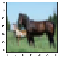

Prior to Deep Learning

Let’s keep in mind our main objective: the Binary classification model.

We already have the training data, now we will load the validation data with the CIFAR10() function and by indicating train=False :

transformed_cifar10_val = datasets.CIFAR10(
    data_path, train=False, download=True,
    transform=transforms.Compose([
        transforms.ToTensor(),
        transforms.Normalize((0.4915, 0.4823, 0.4468),
                             (0.2470, 0.2435, 0.2616))
        ]))

In our dataset there are 10 classes.

We want to do binary classification, so we will keep only 2 of these classes : deer and horse.

Our Deep Learning model will learn to detect these two classes on images.

We extract the images corresponding to these classes from our dataset :

label_map = {4: 0, 7: 1}
class_names = ['deer', 'horse']

cifar2 = [(img, label_map[label])
  for img, label in transformed_cifar10
  if label in [4, 7]]

cifar2_val = [(img, label_map[label])
    for img, label in transformed_cifar10_val
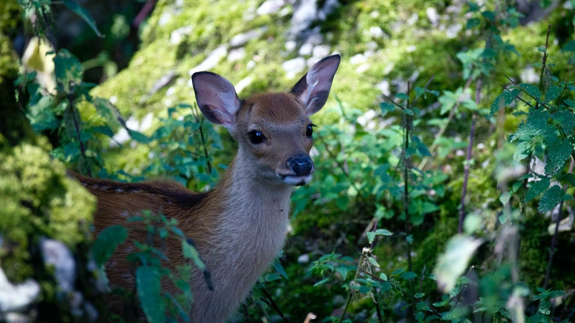
    if label in [4, 7]]

Finally we display one of the images of the class ‘deer’ :

img, ind = cifar2[90]

plt.imshow(unorm(img).permute(1, 2, 0))
plt.show()
print('classe : ', class_names[ind])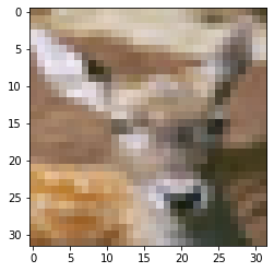

It seems that we are on the right path !

We can continue to the second part of this article with the creation of our Binary Classification model in PyTorch.

sources :

• L. Antiga, Deep Learning with PyTorch (2020, Manning Publications) :
  • our affiliate link – Germany
  • our affiliate link – United Kingdom
• Photo by Diana Parkhouse on Unsplash