Bayesian optimization – What is it? How to use it best?

In this article, I unveil the secrets of Bayesian Optimization, a revolutionary technique for optimizing hyperparameters.

Hyperparameters play an essential role in the performance of Machine Learning models.

However, finding the optimal combination of hyperparameters can be a daunting task. It often requires detailed manual analysis.

But what exactly are these hyperparameters? And how can Bayesian optimization revolutionize their tuning?

Here, I propose to explore the concept of Bayesian optimization, its practice using the bayes_opt library in Python, and its impact on the performance of Machine Learning models.

Hyperparameters

What are Hyperparameters?

Hyperparameters in Machine Learning are configurable elements before a model’s training that influence its behavior and performance.

They should not be confused with the model’s parameters.

The latter are learned from the data during the training of a Machine Learning model and are constantly evolving.

Common hyperparameters include: the learning rate, the depth of a neural network, or the number of branches in a Decision Tree.

By judiciously choosing them, your Machine Learning model can achieve high performance after its training.

The Challenge of Manual Tuning

The choice of hyperparameters can have a significant impact on a model’s performance.

Nevertheless, manually adjusting hyperparameters is time-consuming.

It requires time and often may not have the expected effect.

Indeed, manually adjusting hyperparameters involves:

• running multiple experiments
• iteratively modifying hyperparameters
• evaluating the model’s performance at the end of each experiment

This process can be both tedious and… ineffective ❌

To overcome these limitations, there are now (and have been for a few years) automated optimization techniques.

These methods aim to progressively explore the hyperparameter space in search of the optimal configuration that maximizes a model’s performance.

Bayesian optimization is one of these approaches!🔥

Bayesian Optimization

Introduction to Bayesian Optimization

Bayesian Optimization in Machine Learning is an optimization method that uses probabilistic models to efficiently find a model’s hyperparameters.

In other words, it’s a mathematical technique whose objective is to find the optimal combination of hyperparameters.

This optimization is achieved by intelligently exploring the search space using statistical models.

For this, Bayesian optimization uses:

• a surrogate model
• an acquisition function
• a strategy for balancing exploration and exploitation

Main Components of Bayesian Optimization

The surrogate model allows estimating how the different values of hyperparameters affect the model’s performance.

It uses data from previous experiments to predict the potential performance of new hyperparameter combinations.

Thus, the surrogate model guides the choice of the next configurations to evaluate.

The acquisition function is a mathematical measure that evaluates the interest (or utility) of evaluating a given hyperparameter configuration.

It takes into account both the uncertainty of the surrogate model and the search for an improvement in model performance.

Commonly used acquisition functions include:

• Expected Improvement
• Expected Optimism
• UCB – Upper Confidence Bound

The strategy for balancing exploration and exploitation is the approach used to decide whether to explore new hyperparameter configurations to discover potential improvements (exploration) or exploit currently known configurations considered to be the best (exploitation).

This strategy is essential for efficiently finding the best hyperparameter combination.

To achieve this, it gradually adjusts its approach to choose the next combinations to evaluate based on the optimization goal.

The Iterative Process of Bayesian Optimization

In practice, Bayesian optimization proceeds iteratively:

1. Use the surrogate model to predict the performance of different hyperparameter configurations
2. Use the acquisition function to choose the most promising hyperparameter configuration to evaluate next
3. Evaluate the chosen hyperparameter configuration
4. Update the surrogate model with the new results
5. Repeat the process until a stopping criterion is reached, such as a maximum number of iterations or a satisfactory performance level

The power of Bayesian optimization lies in its ability to use a model to make informed predictions about the parts of the hyperparameter space to explore.

This ability can significantly reduce the number of evaluations needed to find good hyperparameters.

A Library for Bayesian Optimization bayes_opt

bayes_opt is a Python library designed to easily exploit Bayesian optimization.

It is compatible with various Machine Learning libraries, including Scikit-learn and XGBoost. It is therefore a valuable asset for practitioners looking to optimize their models.

This library serves as a bridge between the theoretical foundations of Bayesian optimization and its practical application.

Thus, it adapts the optimization process to specific tasks in Machine Learning.

Let’s see how to use bayes_opt.

Using bayes_opt for Hyperparameter Tuning

Before using the library, it must be installed. This is simply done by using the pip command:

pip install bayesian-optimization==1.3.0

Note: for this tutorial I am using version 1.3.0 of the library.

Now, let’s take a practical example by optimizing the results of a Machine Learning model.

For this example, imagine that we are working on a classification problem using a Random Forest classifier.

In this context, we have several hyperparameters to adjust:

• n_estimators – the number of trees
• max_depth – the maximum depth of the trees
• min_samples_leaf – the minimum number of samples per leaf

Here’s a snippet of Python code demonstrating how to use bayes_opt for hyperparameter optimization with a Random Forest classifier:

from bayes_opt import BayesianOptimization
from sklearn.ensemble import RandomForestClassifier
from sklearn.metrics import accuracy_score
from sklearn.model_selection import cross_val_score

# Define the objective function to optimize
def rf_cv(n_estimators, max_depth, min_samples_leaf):
    model = RandomForestClassifier(
        n_estimators=int(n_estimators),
        max_depth=int(max_depth),
        min_samples_leaf=int(min_samples_leaf),
        random_state=42,
    )
    # Use cross-validation to estimate performance
    scores = cross_val_score(model, X, y, cv=5, scoring='accuracy')
    return scores.mean()

# Create a BayesianOptimization object
bo = BayesianOptimization(
    f=rf_cv,
    pbounds={'n_estimators': (10, 200), 'max_depth': (2, 50), 'min_samples_leaf': (1, 10)},
    verbose=2
)

# Perform the optimization
bo.maximize(init_points=10, n_iter=50, acq='ucb')

# Best hyperparameters and corresponding accuracy
best_params = bo.max['params']
best_accuracy = bo.max['target']

print(f"Best Hyperparameters: {best_params}")
print(f"Best Cross-Validation Accuracy: {best_accuracy}")

The function rf_cv represents the objective. Here, we wish to optimize the average accuracy obtained during the cross-validation of our model.

The variable pbounds defines the search space to explore for selecting hyperparameters.

For this code to work, you must have previously defined the variables X and y.

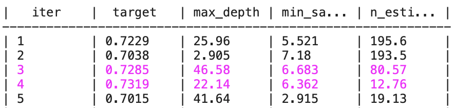
If that’s the case, the result should look like this:

Best Hyperparameters: {'max_depth': 29.597407514950014, 'min_samples_leaf': 8.786274398078726, 'n_estimators': 25.983234732342932}
Best Cross-Validation Accuracy: 0.7341095976398218

Here’s what each column means in this table:

• iter: This is the optimization iteration number. Each iteration represents an attempt to find better hyperparameters.
• target: This is the value of the objective function, the metric for evaluating the model (the average accuracy obtained during the cross-validation).
• max_depth, min_samples_split, n_estimators: These are the values of the hyperparameters explored during Bayesian optimization.

Note: The floating values assigned to integer hyperparameters, such as max_depth and n_estimators, are rounded off when used to obtain an integer.

With each iteration, Bayesian optimization tries a new combination of hyperparameters and records the corresponding performance metric.

When the combination of hyperparameters is better than the previous ones, the line is displayed in purple.

But how do you customize bayes_opt for specific use cases?

Customizing bayes_opt

One of the advantages of bayes_opt is its flexibility. Here are some of the ways you can customize the tool to suit specific needs:

• Define an appropriate objective function: Your objective function can be tailored to different types of metrics such as precision, recall, or F1-score according to the needs of your project (metrics that I have already detailed in this article).
• Use of complex hyperparameter domains: bayes_opt allows specifying domains not only numerical but also categorical if necessary, using techniques such as encoding or mapping.
• Constraints and prerequisites: You can integrate constraints into your search space to discard unviable combinations or to meet certain prerequisites.
• Integration with pipelines: bayes_opt can be integrated into data processing pipelines, allowing you to optimize not only model hyperparameters but also data preprocessing steps.
• Parallelization of optimization: To speed up optimization, bayes_opt can be used with parallelization tools to perform multiple hyperparameter evaluations simultaneously.
• Saving and resuming: It is possible to save the state of optimization and resume optimization later, which is useful for very long optimization processes.
• Visualization of results: bayes_opt can be coupled with visualization libraries to track the progress of optimization and analyze results.

To customize bayes_opt, you can delve into the library’s documentation to understand all the available options.

But for now, here’s an example of how you could extend the existing code to include some of these customizations:

Constraints and Preconditions

# Import necessary libraries for customization
from sklearn.ensemble import RandomForestClassifier
# from sklearn.metrics import accuracy_score
from sklearn.model_selection import cross_val_score
from bayes_opt import BayesianOptimization, UtilityFunction
import numpy as np

# Assume you have a complex model with preconditions such as:
# "max_depth" must not be lower than "min_samples_leaf"
def complex_model_cv(n_estimators, max_depth, min_samples_leaf):
    if max_depth < min_samples_leaf:
        return 0  # An unfavorable return value for unviable combinations
    else:
        model = RandomForestClassifier(
            n_estimators=int(n_estimators),
            max_depth=int(max_depth),
            min_samples_leaf=int(min_samples_leaf),
            random_state=42,
        )
        scores = cross_val_score(model, X, y, cv=5, scoring='accuracy')
        return scores.mean()

# Use UtilityFunction to customize the acquisition function
acq = UtilityFunction(kind="ucb", kappa=2.5, xi=0.0)

# Define a BayesianOptimization object with constraints
pbounds = {'n_estimators': (10, 200), 'max_depth': (2, 50), 'min_samples_leaf': (1, 10)}

bo = BayesianOptimization(
    f=complex_model_cv,
    pbounds=pbounds,
    verbose=2,
)

# Use the custom acquisition function in the optimization process
next_point_to_probe = acq.utility(bo.space.params_to_array(pbounds), bo._gp, bo._random_state)

In this section of code, we initialize a Bayesian optimization process for a RandomForestClassifier using the bayes_opt library.

The model is defined with certain preconditions to avoid non-viable configurations, for instance, the maximum depth of the tree (max_depth) must not be lower than the minimum number of samples required to be at a leaf (min_samples_leaf).

If these conditions are not met, the function returns 0, thus eliminating these hyperparameter combinations from further consideration.

The acquisition function, which guides the selection of the next hyperparameters to test, is customized with UtilityFunction, here using the Upper Confidence Bound (UCB) approach with specific kappa and xi parameters.

This determines the balance between exploiting known well-performing hyperparameters and exploring new hyperparameters.

A BayesianOptimization object is then created with the hyperparameter bounds specified in pbounds. These bounds define the ranges of values within which the optimization should search for the best hyperparameters. Finally, the custom acquisition function is used to determine the next point to evaluate in the hyperparameter space, which is an essential step in the iteration of the Bayesian optimization process.

Saving Optimization

from bayes_opt.logger import JSONLogger
from bayes_opt.event import Events

# Save the optimization state
logger = JSONLogger(path="./logs.log")
bo.subscribe(Events.OPTIMIZATION_STEP, logger)

bo.maximize(init_points=10, n_iter=50, acq='ucb')
params = bo.space.params
target = bo.space.target

This code block illustrates the integration of a logger into bayes_opt, enabling the automatic saving of the optimization state after each step.

The logger is essential for resuming optimization where it left off, particularly for optimization processes that can take a lot of time.

Here, a JSONLogger is attached to the optimizer bo to record events in a log file.

After each optimization step, the best set of hyperparameters is updated, and the current state is saved, which allows for recovery in case of an interruption.

Visualization of Results

import matplotlib.pyplot as plt

# Visualization of optimization
plt.figure(figsize=(8, 2))
plt.scatter(params[:,0], target)
plt.title('N_estimators vs. Target')
plt.xlabel('N_estimators')
plt.ylabel('Target')
plt.show()

# Visualization of optimization convergence
plt.figure(figsize=(8, 2))
plt.plot(np.arange(len(bo.space)), target, '-o')
plt.title('Optimization Convergence')
plt.xlabel('Iteration')
plt.ylabel('Target')
plt.show()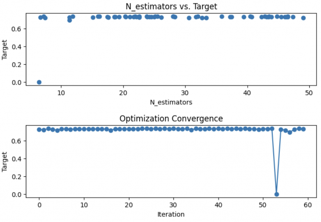

In these lines, we visualize the results of the optimization using matplotlib.

The first chart shows the relationship between the number of estimators and the model performance, helping to identify the optimal number of estimators for our RandomForestClassifier.

The second chart represents the convergence of the optimization over iterations.

It allows checking whether the optimization is progressing towards a better solution or if it is stagnating, which could indicate the need to adjust the optimization process or hyperparameters.

Resuming Optimization

from bayes_opt.util import load_logs

# Define a BayesianOptimization object with constraints
new_bo = BayesianOptimization(
    f=complex_model_cv,
    pbounds=pbounds,
    verbose=2,
)

# Use the custom acquisition function in the optimization process
next_point_to_probe = acq.utility(new_bo.space.params_to_array(pbounds), new_bo._gp, new_bo._random_state)

# The new optimizer is loaded with the previously observed points
load_logs(new_bo, logs=["./logs.log.json"]);

new_bo.maximize(init_points=0, n_iter=20, acq='ucb')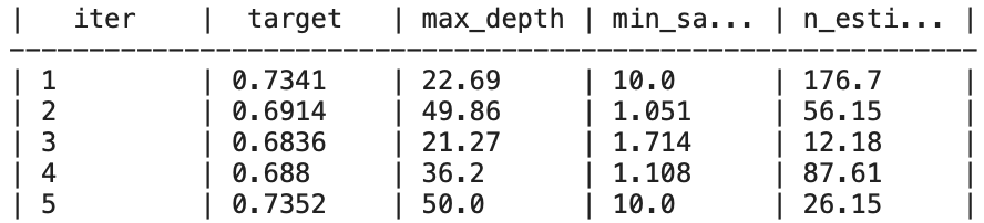

Here, we load the previous optimization state into a new BayesianOptimization object.

Using the load_logs function, we can resume the optimization where it left off, leveraging the information gathered previously.

This is particularly useful for continuing optimization without losing progress made after an interruption. But it can also be useful for starting optimization with a new set of hyperparameters based on previous results.

Going Further

# Best hyperparameters and corresponding accuracy after customization
best_params_custom = new_bo.max['params']
best_accuracy_custom = new_bo.max['target']

print(f"Best Hyperparameters after Customization: {best_params_custom}")
print(f"Best Cross-Validation Accuracy after Customization: {best_accuracy_custom}")

Output:

Best Hyperparameters after Customization: {'max_depth': 7.169316344372172, 'min_samples_leaf': 5.946827832091897, 'n_estimators': 34.972481159917464}
Best Cross-Validation Accuracy after Customization: 0.7374866612265395

The result displays the best hyperparameters obtained after the optimization process with bayes_opt. It also shows the best accuracy achieved using cross-validation. We can then draw a conclusion: Bayesian optimization of hyperparameters has a crucial impact on the model’s performance. The detailed code here shows how to:

• Integrate constraints into your search space with bayes_opt
• Customize the acquisition function to control the balance between exploration and exploitation
• Visualize the progress and results of the optimization
• Save and resume optimization at a certain exploration state

By applying this code on your side, you will see that using bayes_opt works wonders! ✨

To allow you to test this easily – I propose you access a bonus.

Inside, you will find the detailed code above applied to a concrete example.

The data for this experimentation will download automatically, and you will not have to copy the code manually.

You can simply import it into Jupyter, Google Colab, or another, and execute it in one click.

In addition to this, you will access my Action plan to Master Neural networks.

A program of 7 free courses that I have prepared to guide you in your journey to learn Deep Learning.

If the bonus and the program interest you, click here:

GET MY ACTION PLAN