

In this article we share with you the perfect function to train your model with the PyTorch library !
PyTorch is one of the most used libraries for Deep Learning.
This library has the specificity of requiring the developer to code his own functions and classes to train his model.
It is true that PyTorch has a more complex approach but it allows more flexibility, while Keras simplifies our life by making it more standard.
Today I present you this ready to use function to easily train your classification model with PyTorch.
Training PyTorch model
The training function
Here is the function that allows us to train your model while recording the accuracy and loss !
import time

def train(model, optimizer, loss_fn, train_dl, val_dl, epochs=100, device='cpu'):

    print('train() called: model=%s, opt=%s(lr=%f), epochs=%d, device=%s\n' % \
          (type(model).__name__, type(optimizer).__name__,
           optimizer.param_groups[0]['lr'], epochs, device))

    history = {} # Collects per-epoch loss and acc like Keras' fit().
    history['loss'] = []
    history['val_loss'] = []
    history['acc'] = []
    history['val_acc'] = []

    start_time_sec = time.time()

    for epoch in range(1, epochs+1):

        # --- TRAIN AND EVALUATE ON TRAINING SET -----------------------------
        model.train()
        train_loss         = 0.0
        num_train_correct  = 0
        num_train_examples = 0

        for batch in train_dl:

            optimizer.zero_grad()

            x    = batch[0].to(device)
            y    = batch[1].to(device)
            yhat = model(x)
            loss = loss_fn(yhat, y)

            loss.backward()
            optimizer.step()

            train_loss         += loss.data.item() * x.size(0)
            num_train_correct  += (torch.max(yhat, 1)[1] == y).sum().item()
            num_train_examples += x.shape[0]

        train_acc   = num_train_correct / num_train_examples
        train_loss  = train_loss / len(train_dl.dataset)


        # --- EVALUATE ON VALIDATION SET -------------------------------------
        model.eval()
        val_loss       = 0.0
        num_val_correct  = 0
        num_val_examples = 0

        for batch in val_dl:

            x    = batch[0].to(device)
            y    = batch[1].to(device)
            yhat = model(x)
            loss = loss_fn(yhat, y)

            val_loss         += loss.data.item() * x.size(0)
            num_val_correct  += (torch.max(yhat, 1)[1] == y).sum().item()
            num_val_examples += y.shape[0]

        val_acc  = num_val_correct / num_val_examples
        val_loss = val_loss / len(val_dl.dataset)


        if epoch == 1 or epoch % 10 == 0:
          print('Epoch %3d/%3d, train loss: %5.2f, train acc: %5.2f, val loss: %5.2f, val acc: %5.2f' % \
                (epoch, epochs, train_loss, train_acc, val_loss, val_acc))

        history['loss'].append(train_loss)
        history['val_loss'].append(val_loss)
        history['acc'].append(train_acc)
        history['val_acc'].append(val_acc)

    # END OF TRAINING LOOP


    end_time_sec       = time.time()
    total_time_sec     = end_time_sec - start_time_sec
    time_per_epoch_sec = total_time_sec / epochs
    print()
    print('Time total:     %5.2f sec' % (total_time_sec))
    print('Time per epoch: %5.2f sec' % (time_per_epoch_sec))

    return history
Actually this function comes from StackOverflow, a very good site for developers who are wondering about anything.
By the way, if your goal is to master Deep Learning - I've prepared the Action plan to Master Neural networks. for you.
7 days of free advice from an Artificial Intelligence engineer to learn how to master neural networks from scratch:
- Plan your training
- Structure your projects
- Develop your Artificial Intelligence algorithms
I have based this program on scientific facts, on approaches proven by researchers, but also on my own techniques, which I have devised as I have gained experience in the field of Deep Learning.
To access it, click here :
Now we can get back to what I was talking about earlier.
Training your model
To train your model you will need to specify the variables :
- model – torch.nn.Module
- optimizer – torch.optim.Optimizer
- loss_fn – the loss function
- train_dl – DataLoader
- val_dl – DataLoader
- epochs – int
- device – ‘cpu’ or ‘cuda’ to run it with a GPU
history = train(
    model = model,
    optimizer = optimizer,
    loss_fn = loss_fn,
    train_dl = train_loader,
    val_dl = val_loader,
    device='cuda')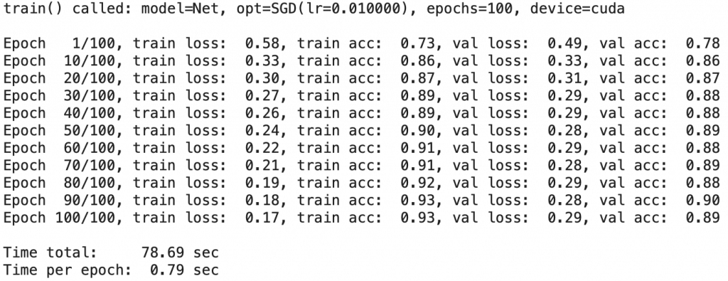
We will have, as an output, a history variable listing the metrics of the model.
Display metrics
To display the performances of the model, you just have to execute this piece of code which uses the matplotlib library to plot the evolution of the model during its training :
import matplotlib.pyplot as plt

acc = history['acc']
val_acc = history['val_acc']
loss = history['loss']
val_loss = history['val_loss']
epochs = range(1, len(acc) + 1)

plt.plot(epochs, acc, 'b', label='Training acc')
plt.plot(epochs, val_acc, 'r', label='Validation acc')
plt.title('Training and validation accuracy')
plt.legend()
plt.figure()
plt.plot(epochs, loss, 'b', label='Training loss')
plt.plot(epochs, val_loss, 'r', label='Validation loss')
plt.title('Training and validation loss')
plt.legend()
plt.show()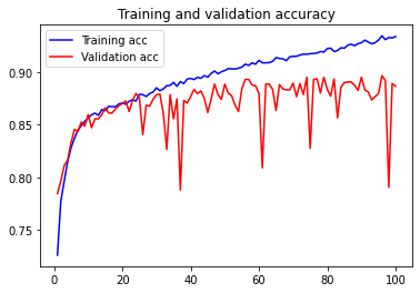
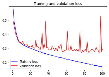
We finally obtain a legible figure with in blue the performances on the training data and in red the performances on the validation data.
It is with this type of figure that we can efficiently analyze if something is wrong with the training of our model !
The training method presented in this article is both fast and efficient but other approaches exist to train your model quickly with PyTorch, notably this extension.
Other libraries such as Keras & TensorFlow offer methods requiring a single code line as explained in this article !
Photo by Shifaaz shamoon on Unsplash
One last word, if you want to go further and learn about Deep Learning - I've prepared for you the Action plan to Master Neural networks. for you.
7 days of free advice from an Artificial Intelligence engineer to learn how to master neural networks from scratch:
- Plan your training
- Structure your projects
- Develop your Artificial Intelligence algorithms
I have based this program on scientific facts, on approaches proven by researchers, but also on my own techniques, which I have devised as I have gained experience in the field of Deep Learning.
To access it, click here :